Problem Solving by Search: Routes, Plans and Paths

Problems as state spaces

A search problem has five parts [1]. The initial state describes where the agent starts. The actions available in a state say what the agent can do. The transition model gives the state that results from an action. The goal test decides whether a state solves the problem, and the path cost adds up the cost of the actions along a sequence. A solution is a sequence of actions from the initial state to a goal state, and an optimal solution has the lowest path cost among all solutions.

The formulation is an engineering decision in its own right. For a haul truck in an open-pit mine, a state can be a node of the road network, and the path cost can be travel time, fuel or tyre wear. For a mobile robot in a factory, the state can be a cell of an occupancy grid, which divides the floor into squares that are free or blocked [2]. For a crane that stacks containers, the state is the arrangement of all containers, and the number of states grows combinatorially. A good formulation keeps only the details that matter for the decision: A route planner for a truck does not need the colour of the truck, but it may need the slope of every road segment.

Uninformed search: Breadth first, depth first and uniform cost

Uninformed strategies know nothing about the goal beyond the goal test. They differ only in the order in which they expand nodes of the search tree. Breadth-first search expands the shallowest node first by keeping the frontier in a first-in first-out queue. It finds the solution with the fewest actions, which is optimal when every action has the same cost. Depth-first search expands the deepest node first with a last-in first-out stack, needs little memory, but may wander along an infinite branch and does not guarantee the shortest solution. Iterative deepening repeats depth-limited search with growing limits and combines the memory use of depth-first search with the completeness of breadth-first search [3].

When actions have different costs, the fewest actions is not the cheapest path. Uniform-cost search expands the node with the lowest path cost so far, which is Dijkstra's algorithm on an explicit graph [4]. It is optimal for non-negative costs, because a node is expanded only when no cheaper route to it can exist.

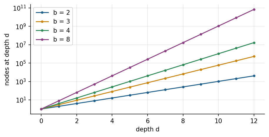
The price of uninformed search is growth. With branching factor b and solution depth d, breadth-first search may generate on the order of b to the power d nodes. On a grid with four moves and a goal forty steps away, blind search explores almost every reachable cell within that radius. The number becomes unmanageable for combinatorial problems such as sequencing: Twenty jobs can be ordered in more than two quintillion ways.

Informed search: Heuristics and A*

A heuristic function h(n) estimates the cost from node n to the nearest goal. Greedy best-first search expands the node with the smallest h and often reaches a goal quickly, but it can be misled into long detours. A* combines the cost already paid, g(n), with the estimate, and expands the node with the smallest f(n) = g(n) + h(n) [5].

Hart, Nilsson and Raphael showed that A returns an optimal path if the heuristic is admissible, which means it never overestimates the true remaining cost [5]. The straight-line distance is admissible for road travel, because no road is shorter than a straight line. On a grid with four moves, the Manhattan distance, the sum of horizontal and vertical offsets, is admissible. A heuristic is consistent when its estimate never drops by more than the cost of one step. Consistency implies admissibility and guarantees that A never needs to reopen a node [6].

Better heuristics save work. If one admissible heuristic is always at least as large as another, A with the larger one expands no more nodes. The zero heuristic turns A into uniform-cost search, and a perfect heuristic walks straight to the goal. Weighted A* multiplies the heuristic by a factor larger than one: It usually expands far fewer nodes and returns a path whose cost is at most that factor times the optimum, which is a common engineering compromise when planning must meet a deadline.

Path planning for vehicles and machines

Path planning in engineering adds physical constraints to graph search. Occupancy grids and road graphs give the search space, while costs encode travel time, energy, risk or wear [2]. Vehicles cannot turn on the spot, so planners for cars and trucks search over positions and headings. Hybrid A* keeps continuous positions inside discrete cells and has been used to park and manoeuvre autonomous vehicles in unstructured environments such as parking lots [7]. Surveys of self-driving urban vehicles place such graph-search planners next to sampling-based and optimisation-based methods [8].

Terrain adds cost and feasibility. A haul road in a mine, a pipeline or a forest road must respect a maximum grade, and steep segments cost more fuel and time. A digital elevation model turns the terrain into a grid of heights, and the cost of moving between two cells can combine distance with a penalty on slope and a hard limit above which the move is forbidden. The notebook applies this idea to a real elevation grid near Isparta from the Copernicus GLO-90 model, served by the Open-Meteo Elevation API [9, 10].

Beyond systematic search: Local search

Systematic search remembers the paths it explores. Local search keeps only a current solution and improves it by small changes, which suits problems where the path does not matter and only the final configuration counts, such as a layout or a schedule. Hill climbing accepts only improvements and stops at the first local optimum. Simulated annealing sometimes accepts worse solutions, with a probability that falls as a temperature parameter is lowered, and can therefore escape local optima [11]. Weeks 5 and 6 develop this line into evolutionary and swarm algorithms, which keep a population of candidate solutions instead of one.

Review cards

Select a card to turn it over.

References

[1] Russell, S., & Norvig, P. (2021). Artificial Intelligence: A Modern Approach (4th ed.). Pearson.
[2] LaValle, S. M. (2006). Planning Algorithms. Cambridge University Press. https://doi.org/10.1017/CBO9780511546877
[3] Korf, R. E. (1985). Depth-first iterative-deepening: An optimal admissible tree search. Artificial Intelligence, 27(1), 97-109. https://doi.org/10.1016/0004-3702(85)90084-0
[4] Dijkstra, E. W. (1959). A note on two problems in connexion with graphs. Numerische Mathematik, 1, 269-271. https://doi.org/10.1007/BF01386390
[5] Hart, P. E., Nilsson, N. J., & Raphael, B. (1968). A formal basis for the heuristic determination of minimum cost paths. IEEE Transactions on Systems Science and Cybernetics, 4(2), 100-107. https://doi.org/10.1109/TSSC.1968.300136
[6] Pearl, J. (1984). Heuristics: Intelligent Search Strategies for Computer Problem Solving. Addison-Wesley.
[7] Dolgov, D., Thrun, S., Montemerlo, M., & Diebel, J. (2010). Path planning for autonomous vehicles in unknown semi-structured environments. The International Journal of Robotics Research, 29(5), 485-501. https://doi.org/10.1177/0278364909359210
[8] Paden, B., Čáp, M., Yong, S. Z., Yershov, D., & Frazzoli, E. (2016). A survey of motion planning and control techniques for self-driving urban vehicles. IEEE Transactions on Intelligent Vehicles, 1(1), 33-55. https://doi.org/10.1109/TIV.2016.2578706
[9] European Space Agency (2021). Copernicus Global Digital Elevation Model (GLO-90). https://doi.org/10.5270/ESA-c5d3d65
[10] Open-Meteo (2026). Open-Meteo free weather API: Historical Weather API and Elevation API (data licensed under CC BY 4.0). https://open-meteo.com
[11] Kirkpatrick, S., Gelatt, C. D., & Vecchi, M. P. (1983). Optimization by simulated annealing. Science, 220(4598), 671-680. https://doi.org/10.1126/science.220.4598.671