Evolutionary Computation for Engineering Design

Optimisation problems in engineering design

An optimisation problem has design variables, an objective to minimise or maximise, and constraints that a design must satisfy. For a beam, the variables may be the width and height of the cross-section, the objective its mass, and the constraints limits on stress and deflection. Many engineering objectives are black boxes: They are evaluated by a simulation, have no usable gradient, are noisy, or mix continuous and integer variables. Landscapes with many local optima defeat gradient methods that start from a single point.

Population-based metaheuristics address these difficulties by sampling many designs at once and moving the population towards better regions. They make few assumptions about the problem, which is their strength and their limit: The no free lunch theorems show that, averaged over all possible problems, no search algorithm outperforms any other [1]. An algorithm performs well only when its search behaviour matches the structure of the problem, so engineering knowledge about variables, scales and constraints remains decisive.

Genetic algorithms

Holland described adaptation in natural and artificial systems as the evolution of a population under selection and recombination [2], and Goldberg popularised genetic algorithms as practical search and optimisation tools [3]. A genetic algorithm encodes a design as a chromosome, which may be a bit string, a vector of real numbers or a permutation. A fitness function scores each chromosome. Selection chooses parents with a preference for fitter individuals: In tournament selection, a few individuals are drawn at random and the best of them becomes a parent. Crossover combines two parents into offspring, for example by exchanging parts of their chromosomes or by blending their real values. Mutation makes small random changes that keep diversity in the population. Elitism copies the best individuals unchanged into the next generation, so that the best design found is never lost.

The balance between exploration and exploitation governs performance. Strong selection pressure and small mutations converge quickly but risk premature convergence to a local optimum; weak pressure and large mutations explore widely but converge slowly. Population size, tournament size, crossover and mutation rates are therefore design parameters of the algorithm itself, and their effect must be judged over several independent runs, because a single run of a stochastic algorithm proves little [4].

Differential evolution and other real-valued methods

Differential evolution, proposed by Storn and Price, is a simple and effective method for continuous variables [5]. For each member of the population it builds a mutant vector by adding a scaled difference of two random members to a third, v = a + F (b - c), mixes the mutant with the current member by crossover with rate CR, and keeps the trial vector only if it is at least as good. Because the differences between population members shrink as the population converges, the step size adapts automatically to the scale of the landscape. SciPy provides a mature implementation with bounds and constraints [6].

Evolution strategies adapt a distribution of mutations instead. The covariance matrix adaptation evolution strategy, CMA-ES, learns the shape of promising regions and is among the most reliable methods for difficult continuous problems of moderate dimension [7]. Simulated annealing, met in Week 2, is a single-solution relative of these methods [8].

Constraints

Engineering designs must be feasible. A penalty function adds to the objective a term that grows with the amount of constraint violation, which turns a constrained problem into an unconstrained one; the difficulty is choosing the weight of the penalty. Deb's feasibility rules avoid weights altogether: A feasible design always beats an infeasible one, two feasible designs are compared by objective, and two infeasible designs are compared by their total violation [9]. Repair operators that move an infeasible design back into the feasible region are useful when the constraint structure is known, and variable bounds are usually enforced directly.

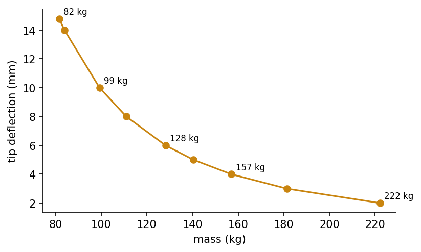
For the cantilever beam of the notebook, a tip load P acts on a rectangular section of width b and height h. The maximum bending stress is 6 P L / (b h squared) and the tip deflection is 4 P L cubed / (E b h cubed) [10]. Minimising mass subject to limits on stress, deflection and the ratio h / b produces an optimum on the boundary of the feasible region, where the deflection limit and the ratio limit are both active. This optimum can be derived by hand, which makes the problem a good benchmark for the algorithms.

Multiple objectives and Pareto optimality

Real designs trade off several objectives: mass against stiffness, cost against reliability, efficiency against noise. A design dominates another if it is no worse in every objective and better in at least one. The designs that no other design dominates form the Pareto set, and their objective values form the Pareto front. The engineer, not the algorithm, chooses a design from the front by weighing the objectives. NSGA-II finds approximations of the front in one run by ranking the population into non-dominated fronts and preserving spread with a crowding distance [11]. Simpler methods repeat single-objective optimisation, for example minimising mass for a sequence of deflection limits, which is how the notebook builds its front.

Evolution at work

Evolutionary computation has produced designs that engineers would hardly have proposed by hand. An X-band antenna evolved at NASA for the Space Technology 5 mission met demanding requirements and flew in space in 2006 [12]. Structural shapes, truss topologies, electrical machines, chemical process conditions and production schedules are routinely optimised with genetic algorithms, differential evolution and their relatives [4]. Week 6 continues with swarm intelligence, which replaces biological evolution by the collective behaviour of birds, ants and bees.

Review cards

Select a card to turn it over.

References

[1] Wolpert, D. H., & Macready, W. G. (1997). No free lunch theorems for optimization. IEEE Transactions on Evolutionary Computation, 1(1), 67-82. https://doi.org/10.1109/4235.585893
[2] Holland, J. H. (1992). Adaptation in Natural and Artificial Systems (2nd ed.). MIT Press. First edition 1975, University of Michigan Press.
[3] Goldberg, D. E. (1989). Genetic Algorithms in Search, Optimization, and Machine Learning. Addison-Wesley.
[4] Eiben, A. E., & Smith, J. E. (2015). Introduction to Evolutionary Computing (2nd ed.). Springer. https://doi.org/10.1007/978-3-662-44874-8
[5] Storn, R., & Price, K. (1997). Differential evolution: A simple and efficient heuristic for global optimization over continuous spaces. Journal of Global Optimization, 11(4), 341-359. https://doi.org/10.1023/A:1008202821328
[6] Virtanen, P., Gommers, R., Oliphant, T. E., et al. (2020). SciPy 1.0: Fundamental algorithms for scientific computing in Python. Nature Methods, 17(3), 261-272. https://doi.org/10.1038/s41592-019-0686-2
[7] Hansen, N., & Ostermeier, A. (2001). Completely derandomized self-adaptation in evolution strategies. Evolutionary Computation, 9(2), 159-195. https://doi.org/10.1162/106365601750190398
[8] Kirkpatrick, S., Gelatt, C. D., & Vecchi, M. P. (1983). Optimization by simulated annealing. Science, 220(4598), 671-680. https://doi.org/10.1126/science.220.4598.671
[9] Deb, K. (2000). An efficient constraint handling method for genetic algorithms. Computer Methods in Applied Mechanics and Engineering, 186(2-4), 311-338. https://doi.org/10.1016/S0045-7825(99)00389-8
[10] Gere, J. M., & Goodno, B. J. (2013). Mechanics of Materials (8th ed.). Cengage Learning.
[11] Deb, K., Pratap, A., Agarwal, S., & Meyarivan, T. (2002). A fast and elitist multiobjective genetic algorithm: NSGA-II. IEEE Transactions on Evolutionary Computation, 6(2), 182-197. https://doi.org/10.1109/4235.996017
[12] Hornby, G. S., Lohn, J. D., & Linden, D. S. (2011). Computer-automated evolution of an X-band antenna for NASA's Space Technology 5 mission. Evolutionary Computation, 19(1), 1-23. https://doi.org/10.1162/EVCO_a_00005