Classification and Evaluation: Defects, Failures and Grades

Classification problems in engineering

A classifier assigns an input to one of several classes. Quality inspection separates good from defective parts, condition monitoring distinguishes fault modes, food engineering grades products, and geology assigns facies to depth intervals of a well. A classifier divides the input space into regions separated by decision boundaries. Most modern classifiers do more than name a class: They estimate a probability or a score for each class, and a decision rule, usually a threshold, turns the score into an action. Separating the model from the decision is essential in engineering, because the costs of different mistakes are rarely equal.

Models for classification

Logistic regression models the log-odds of a class as a linear function of the inputs, so its decision boundary is a straight line or a plane, and its coefficients show the direction in which each input pushes the decision [1]. The k-nearest-neighbour classifier takes a vote among the most similar training examples [2]. Support vector machines find the boundary with the largest margin between classes and use kernels to draw curved boundaries in the original space [3]. Decision trees ask a sequence of threshold questions and are easy to read [4, 5]; random forests and gradient boosting combine many trees and are among the strongest methods for tabular engineering data [6, 7].

The confusion matrix and its metrics

For a binary problem with a positive class, such as "failure", the confusion matrix counts true positives (TP), false positives (FP), false negatives (FN) and true negatives (TN). Accuracy, the share of correct decisions, is misleading when classes are imbalanced: If 3 percent of machines fail, a model that always predicts "no failure" is 97 percent accurate and useless. Precision, TP / (TP + FP), is the share of alarms that are real. Recall, TP / (TP + FN), is the share of real failures that are caught. The F1 score is their harmonic mean. For several classes, the metrics are computed per class and averaged, either equally for every class (macro average) or weighted by class size (weighted average); the macro average reveals poor performance on small classes.

Curves, thresholds and costs

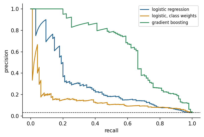
Varying the threshold traces curves. The ROC curve plots the true positive rate against the false positive rate, and the area under it (AUC) equals the probability that a random positive example receives a higher score than a random negative one [8]. When positives are rare, the precision-recall curve is more informative, because the false positive rate can look small while alarms are still mostly false [9].

The threshold should come from the application. If a missed bearing failure costs twenty times more than an unnecessary inspection, the expected cost for each threshold on validation data can be computed, and the threshold with the lowest cost chosen. The default of 0.5 is only correct when both errors cost the same and the probabilities are well calibrated.

Imbalanced data

Rare events are the rule in engineering: failures, defects, accidents, rock bursts. Several remedies exist. Stratified splits keep the class proportions equal in training and test data. Class weights make errors on the rare class more expensive during training. Resampling duplicates rare examples or removes common ones, and SMOTE creates synthetic minority examples by interpolating between neighbouring minority samples [10]. None of these remedies creates information; the most effective step is often better features, more minority data or a problem definition that matches the decision.

Explaining classifiers

Engineers need to know why a model decides. Permutation importance measures how much a performance metric drops when the values of one feature are shuffled, which breaks its link to the target. SHAP values distribute a single prediction among the features according to a game-theoretic rule and are widely used for tree ensembles [11]. In predictive maintenance, explanations connect model output to physical mechanisms such as heat dissipation or tool wear [12]. Newer methods study the geometry of a model's decision function, for example GEMEX, which the instructor developed as an open Python package [13]. Explanations are models of models and can mislead, so they should be checked against domain knowledge and, where possible, against deliberately constructed test cases.

Review cards

Select a card to turn it over.

References

[1] Hastie, T., Tibshirani, R., & Friedman, J. (2009). The Elements of Statistical Learning: Data Mining, Inference, and Prediction (2nd ed.). Springer. https://doi.org/10.1007/978-0-387-84858-7
[2] Cover, T., & Hart, P. (1967). Nearest neighbor pattern classification. IEEE Transactions on Information Theory, 13(1), 21-27. https://doi.org/10.1109/TIT.1967.1053964
[3] Cortes, C., & Vapnik, V. (1995). Support-vector networks. Machine Learning, 20(3), 273-297. https://doi.org/10.1007/BF00994018
[4] Breiman, L., Friedman, J. H., Olshen, R. A., & Stone, C. J. (1984). Classification and Regression Trees. Wadsworth.
[5] Quinlan, J. R. (1986). Induction of decision trees. Machine Learning, 1(1), 81-106. https://doi.org/10.1007/BF00116251
[6] Breiman, L. (2001). Random forests. Machine Learning, 45(1), 5-32. https://doi.org/10.1023/A:1010933404324
[7] Chen, T., & Guestrin, C. (2016). XGBoost: A scalable tree boosting system. In Proceedings of the 22nd ACM SIGKDD International Conference on Knowledge Discovery and Data Mining (pp. 785-794). https://doi.org/10.1145/2939672.2939785
[8] Fawcett, T. (2006). An introduction to ROC analysis. Pattern Recognition Letters, 27(8), 861-874. https://doi.org/10.1016/j.patrec.2005.10.010
[9] Saito, T., & Rehmsmeier, M. (2015). The precision-recall plot is more informative than the ROC plot when evaluating binary classifiers on imbalanced datasets. PLOS ONE, 10(3), e0118432. https://doi.org/10.1371/journal.pone.0118432
[10] Chawla, N. V., Bowyer, K. W., Hall, L. O., & Kegelmeyer, W. P. (2002). SMOTE: Synthetic minority over-sampling technique. Journal of Artificial Intelligence Research, 16, 321-357. https://doi.org/10.1613/jair.953
[11] Lundberg, S. M., & Lee, S.-I. (2017). A unified approach to interpreting model predictions. In Advances in Neural Information Processing Systems 30 (pp. 4765-4774). https://arxiv.org/abs/1705.07874
[12] Matzka, S. (2020). Explainable artificial intelligence for predictive maintenance applications. In 2020 Third International Conference on Artificial Intelligence for Industries (AI4I) (pp. 69-74). IEEE. https://doi.org/10.1109/AI4I49448.2020.00023
[13] Kose, U. (2026). GEMEX: Geodesic Entropic Manifold Explainability (Version 1.2.2) [Python package]. Python Package Index. https://pypi.org/project/gemex/