Patterns without Labels: Clustering, Signals and Anomaly Detection

Learning without labels

Supervised learning needs a label for every example. In engineering, labels are expensive: A geologist must interpret each metre of a well, a technician must confirm each fault, and many rare events have never been observed. Unsupervised learning works with the inputs alone. Clustering groups similar records, dimensionality reduction summarises many correlated variables with a few, and anomaly detection flags records that differ from the bulk of the data [1, 2]. The results are hypotheses that domain experts must interpret: A cluster is not a rock type, and an anomaly is not a fault, until someone checks.

k-means and the choice of k

k-means represents each cluster by a centre and alternates two steps: assign every point to its nearest centre, then move every centre to the mean of its points. Each step lowers the sum of squared distances, so the procedure converges, although only to a local optimum [3, 4]. The k-means++ initialisation spreads the initial centres out and improves both speed and quality [5]. Because k-means uses Euclidean distance, inputs with large numerical ranges dominate unless they are scaled; gamma-ray counts in API units would otherwise swamp a photoelectric factor.

The number of clusters is a modelling choice. The within-cluster sum of squares always falls as k grows, so the elbow of its curve is only a rough guide. The silhouette of a point compares its mean distance to its own cluster with that to the nearest other cluster, and the average silhouette over all points is highest for well-separated, compact clusters [6]. Neither criterion knows the physics; well logs may form five clear clusters although geologists distinguish nine facies.

Principal component analysis

Principal component analysis finds orthogonal directions along which the data vary most [7, 8]. The first component is the direction of largest variance, the second the largest remaining variance orthogonal to the first, and so on. The explained variance ratio of each component shows how much information a projection keeps, and the loadings show how each original variable contributes. In well logging, the first components often combine porosity and density logs, which respond to the same rock properties. PCA serves visualisation, compression, noise reduction and the detection of anomalies as points that the leading components reconstruct poorly.

Density-based clustering

Clusters in engineering data are not always round. Earthquakes line up along faults, defects form streaks on a web of fabric, and traffic accidents gather along roads. DBSCAN defines clusters as regions of high density: A point with at least a minimum number of neighbours within a radius eps is a core point, clusters grow by connecting core points that are neighbours, and points that belong to no cluster are labelled noise [9]. DBSCAN finds clusters of arbitrary shape and does not need the number of clusters, but eps and the minimum number of points must fit the density of the data. For epicentres, distances should be measured on the sphere, for example with the haversine formula, rather than in degrees.

Signals in the frequency domain

Many engineering sensors produce time series sampled at a fixed rate: accelerometers on machines, microphones, current transducers, seismometers. The discrete Fourier transform expresses a sampled signal as a sum of sinusoids, and the fast Fourier transform computes it efficiently [10]. The sampling rate fs limits the highest frequency that can be represented to fs / 2, the Nyquist frequency, and a record of duration T resolves frequencies that differ by 1 / T. Rotating machines produce peaks at the shaft frequency and its harmonics, and faults add their own frequencies.

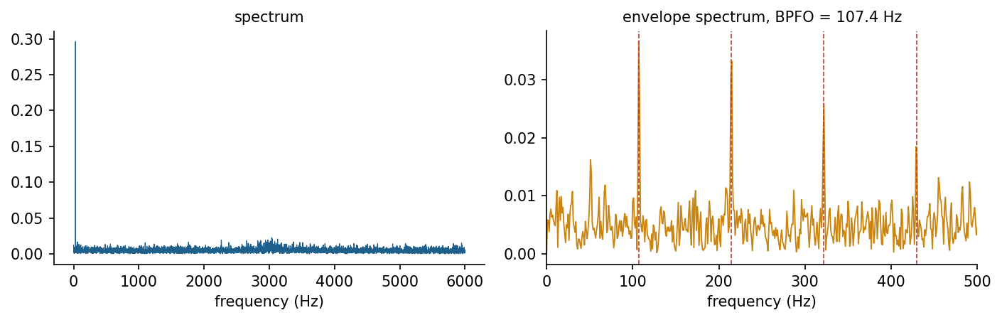
A rolling-element bearing with a damaged outer race produces an impact every time a rolling element passes the damage. The ball pass frequency of the outer race is BPFO = (n / 2) fr (1 - (d / D) cos phi), with n rolling elements of diameter d, pitch diameter D, contact angle phi and shaft frequency fr. The impacts excite structural resonances at high frequency, so the fault frequency often appears not in the raw spectrum but in the spectrum of the signal's envelope, obtained after demodulation. Envelope analysis is the benchmark technique of bearing diagnostics [11], and the Case Western Reserve University data are the standard test set for it [12]. Simple condition indicators complement spectra: the root mean square (RMS) measures vibration energy, kurtosis measures impulsiveness, and the crest factor compares the peak with the RMS.

Anomaly detection

An anomaly detector learns what normal data look like and scores how unusual a new record is [2]. Statistical rules flag values far from the mean in units of standard deviation. Reconstruction-based methods flag records that a PCA model or an autoencoder reconstructs poorly. Isolation forests grow random trees that split the data at random thresholds; anomalies are isolated after few splits, so the average path length to isolate a point becomes its score [13]. In condition monitoring, detectors are usually trained on data from normal operation, because faults are rare and diverse. The alarm threshold, as in Week 8, depends on the costs of false alarms and missed faults, and a detector must be re-examined when operating conditions change, since a new load or speed can look like an anomaly [14].

Review cards

Select a card to turn it over.

References

[1] Hastie, T., Tibshirani, R., & Friedman, J. (2009). The Elements of Statistical Learning: Data Mining, Inference, and Prediction (2nd ed.). Springer. https://doi.org/10.1007/978-0-387-84858-7
[2] Chandola, V., Banerjee, A., & Kumar, V. (2009). Anomaly detection: A survey. ACM Computing Surveys, 41(3), 15. https://doi.org/10.1145/1541880.1541882
[3] Lloyd, S. (1982). Least squares quantization in PCM. IEEE Transactions on Information Theory, 28(2), 129-137. https://doi.org/10.1109/TIT.1982.1056489
[4] MacQueen, J. (1967). Some methods for classification and analysis of multivariate observations. In Proceedings of the Fifth Berkeley Symposium on Mathematical Statistics and Probability, Vol. 1 (pp. 281-297). University of California Press.
[5] Arthur, D., & Vassilvitskii, S. (2007). k-means++: The advantages of careful seeding. In Proceedings of the Eighteenth Annual ACM-SIAM Symposium on Discrete Algorithms (pp. 1027-1035). SIAM.
[6] Rousseeuw, P. J. (1987). Silhouettes: A graphical aid to the interpretation and validation of cluster analysis. Journal of Computational and Applied Mathematics, 20, 53-65. https://doi.org/10.1016/0377-0427(87)90125-7
[7] Pearson, K. (1901). On lines and planes of closest fit to systems of points in space. The London, Edinburgh, and Dublin Philosophical Magazine and Journal of Science, 2(11), 559-572. https://doi.org/10.1080/14786440109462720
[8] Jolliffe, I. T., & Cadima, J. (2016). Principal component analysis: A review and recent developments. Philosophical Transactions of the Royal Society A, 374(2065), 20150202. https://doi.org/10.1098/rsta.2015.0202
[9] Ester, M., Kriegel, H.-P., Sander, J., & Xu, X. (1996). A density-based algorithm for discovering clusters in large spatial databases with noise. In Proceedings of the Second International Conference on Knowledge Discovery and Data Mining (KDD-96) (pp. 226-231). AAAI Press.
[10] Cooley, J. W., & Tukey, J. W. (1965). An algorithm for the machine calculation of complex Fourier series. Mathematics of Computation, 19(90), 297-301. https://doi.org/10.1090/S0025-5718-1965-0178586-1
[11] Randall, R. B., & Antoni, J. (2011). Rolling element bearing diagnostics: A tutorial. Mechanical Systems and Signal Processing, 25(2), 485-520. https://doi.org/10.1016/j.ymssp.2010.07.017
[12] Smith, W. A., & Randall, R. B. (2015). Rolling element bearing diagnostics using the Case Western Reserve University data: A benchmark study. Mechanical Systems and Signal Processing, 64-65, 100-131. https://doi.org/10.1016/j.ymssp.2015.04.021
[13] Liu, F. T., Ting, K. M., & Zhou, Z.-H. (2008). Isolation forest. In 2008 Eighth IEEE International Conference on Data Mining (pp. 413-422). https://doi.org/10.1109/ICDM.2008.17
[14] Lei, Y., Yang, B., Jiang, X., Jia, F., Li, N., & Nandi, A. K. (2020). Applications of machine learning to machine fault diagnosis: A review and roadmap. Mechanical Systems and Signal Processing, 138, 106587. https://doi.org/10.1016/j.ymssp.2019.106587