Seeing with Networks: Convolutional Neural Networks and Computer Vision

Images as engineering data

A digital image is an array of numbers. A greyscale image of 64 by 64 pixels holds 4096 intensities, and a colour image stores three such arrays, one per channel. Engineering images come from inspection cameras on production lines, drones over bridges and power lines, microscopes, satellites, thermal cameras and X-ray systems. Treating the pixels as 4096 unrelated inputs to a multilayer network ignores two facts: Neighbouring pixels belong together, and the same pattern, such as an edge or a crack, can appear anywhere in the image. Convolutional networks build both facts into their structure.

Convolution, feature maps and pooling

A convolutional layer slides a small filter, for example 3 by 3 weights, over the image and computes at every position the weighted sum of the pixels under it. The result is a feature map that is large where the image locally resembles the filter. A vertical-edge filter responds to vertical edges wherever they are, because the same weights are used at every position. This weight sharing drastically reduces the number of parameters compared with a fully connected layer and makes the detector equivariant to shifts [1, 2]. A layer learns many filters at once, each producing its own feature map, or channel.

Three settings shape a convolution. The kernel size sets the local window, the stride sets the step between positions, and padding adds a border so that the output can keep the input size. For an input of width W, kernel K, padding P and stride S, the output width is (W - K + 2P) / S + 1. Pooling layers then summarise small neighbourhoods, usually by their maximum, which halves the resolution and makes the representation more tolerant to small shifts. Stacking convolution, activation and pooling lets later layers see larger parts of the image: Early layers detect edges and textures, later layers combine them into parts and objects [3].

Deep architectures

LeNet showed in the 1990s that convolutional networks trained by backpropagation read handwritten digits reliably [2]. AlexNet, a deeper network trained on graphics processors with ReLU activations and dropout, won the 2012 ImageNet challenge by a wide margin [4, 5]. VGG networks used only small 3 by 3 filters stacked deeply [6]. Residual networks added shortcut connections that let a layer learn a correction to its input, which made networks with more than a hundred layers trainable [7]. Vision transformers split an image into patches and process them with the attention mechanism of Week 13; with enough data they match or exceed convolutional networks [8].

Training with little data

Engineering datasets are small compared with ImageNet: a few hundred labelled crack photographs, a few thousand defect images. Two techniques make deep networks usable nonetheless. Data augmentation creates plausible variants of the training images by flipping, rotating, cropping or changing brightness, which teaches invariances that the task requires. Transfer learning starts from a network pretrained on a large dataset and retrains only its last layers or fine-tunes all of them with a small learning rate; Yosinski and colleagues showed that early layers learn general features that transfer well between tasks [9]. Cha and colleagues trained a convolutional network on patches of concrete photographs to detect cracks under varied lighting [10], and similar studies inspect steel strip surfaces [11], crops and weeds [12] and traffic signs [13].

Beyond classification

Classification assigns one label to an image. Object detection finds and labels every object with a bounding box; YOLO treats detection as a single regression problem and runs in real time [14]. Semantic segmentation labels every pixel; U-Net combines a contracting path with an expanding path and skip connections and became a standard for segmentation with few training images [15]. For a bridge inspector, a classifier says "crack present", a detector draws a box around each crack, and a segmentation network outlines the crack so that its length and width can be measured.

Seeing what the network sees

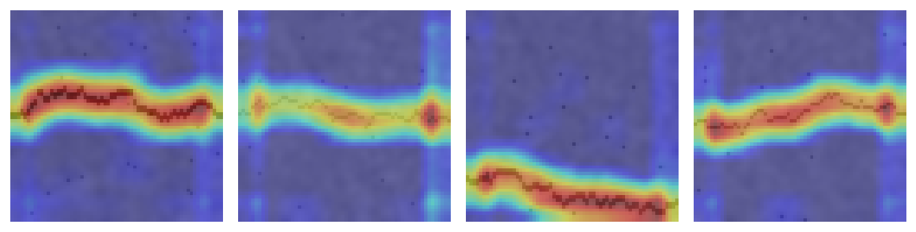
High accuracy does not prove that a network uses the right evidence. A defect classifier may learn the lighting of the station where defective parts were photographed, or the ruler that appears only in images of damaged specimens. Grad-CAM weighs the feature maps of the last convolutional layer by the gradient of the class score and produces a coarse heatmap of the regions that drove the decision [16]. Checking such maps on a sample of test images, and testing the network on images from new cameras and sites, belongs to every engineering deployment. Vision models are also vulnerable to small, deliberate perturbations of the input that change their decisions, which matters wherever an attacker could manipulate the images [17].

Review cards

Select a card to turn it over.

References

[1] LeCun, Y., Boser, B., Denker, J. S., et al. (1989). Backpropagation applied to handwritten zip code recognition. Neural Computation, 1(4), 541-551. https://doi.org/10.1162/neco.1989.1.4.541
[2] LeCun, Y., Bottou, L., Bengio, Y., & Haffner, P. (1998). Gradient-based learning applied to document recognition. Proceedings of the IEEE, 86(11), 2278-2324. https://doi.org/10.1109/5.726791
[3] LeCun, Y., Bengio, Y., & Hinton, G. (2015). Deep learning. Nature, 521(7553), 436-444. https://doi.org/10.1038/nature14539
[4] Krizhevsky, A., Sutskever, I., & Hinton, G. E. (2017). ImageNet classification with deep convolutional neural networks. Communications of the ACM, 60(6), 84-90. https://doi.org/10.1145/3065386
[5] Deng, J., Dong, W., Socher, R., Li, L.-J., Li, K., & Fei-Fei, L. (2009). ImageNet: A large-scale hierarchical image database. In 2009 IEEE Conference on Computer Vision and Pattern Recognition (pp. 248-255). https://doi.org/10.1109/CVPR.2009.5206848
[6] Simonyan, K., & Zisserman, A. (2015). Very deep convolutional networks for large-scale image recognition. In 3rd International Conference on Learning Representations (ICLR 2015). https://arxiv.org/abs/1409.1556
[7] He, K., Zhang, X., Ren, S., & Sun, J. (2016). Deep residual learning for image recognition. In 2016 IEEE Conference on Computer Vision and Pattern Recognition (CVPR) (pp. 770-778). https://doi.org/10.1109/CVPR.2016.90
[8] Dosovitskiy, A., Beyer, L., Kolesnikov, A., et al. (2021). An image is worth 16x16 words: Transformers for image recognition at scale. In 9th International Conference on Learning Representations (ICLR 2021). https://arxiv.org/abs/2010.11929
[9] Yosinski, J., Clune, J., Bengio, Y., & Lipson, H. (2014). How transferable are features in deep neural networks?. In Advances in Neural Information Processing Systems 27 (pp. 3320-3328). https://arxiv.org/abs/1411.1792
[10] Cha, Y.-J., Choi, W., & Büyüköztürk, O. (2017). Deep learning-based crack damage detection using convolutional neural networks. Computer-Aided Civil and Infrastructure Engineering, 32(5), 361-378. https://doi.org/10.1111/mice.12263
[11] Song, K., & Yan, Y. (2013). A noise robust method based on completed local binary patterns for hot-rolled steel strip surface defects. Applied Surface Science, 285, 858-864. https://doi.org/10.1016/j.apsusc.2013.09.002
[12] Kamilaris, A., & Prenafeta-Boldú, F. X. (2018). Deep learning in agriculture: A survey. Computers and Electronics in Agriculture, 147, 70-90. https://doi.org/10.1016/j.compag.2018.02.016
[13] Stallkamp, J., Schlipsing, M., Salmen, J., & Igel, C. (2012). Man vs. computer: Benchmarking machine learning algorithms for traffic sign recognition. Neural Networks, 32, 323-332. https://doi.org/10.1016/j.neunet.2012.02.016
[14] Redmon, J., Divvala, S., Girshick, R., & Farhadi, A. (2016). You only look once: Unified, real-time object detection. In 2016 IEEE Conference on Computer Vision and Pattern Recognition (CVPR) (pp. 779-788). https://doi.org/10.1109/CVPR.2016.91
[15] Ronneberger, O., Fischer, P., & Brox, T. (2015). U-Net: Convolutional networks for biomedical image segmentation. In Medical Image Computing and Computer-Assisted Intervention (MICCAI 2015), LNCS 9351 (pp. 234-241). Springer. https://doi.org/10.1007/978-3-319-24574-4_28
[16] Selvaraju, R. R., Cogswell, M., Das, A., Vedantam, R., Parikh, D., & Batra, D. (2017). Grad-CAM: Visual explanations from deep networks via gradient-based localization. In 2017 IEEE International Conference on Computer Vision (ICCV) (pp. 618-626). https://doi.org/10.1109/ICCV.2017.74
[17] Kose, U. (2019). Techniques for adversarial examples threatening the safety of artificial intelligence based systems. In I. International Science and Innovation Congress (INSI Congress 2019). Pamukkale, Denizli, Türkiye. https://arxiv.org/abs/1910.06907