Overview
Reinforcement learning is learning from interaction: An agent acts, the environment answers with a new situation and a reward, and the agent improves its behaviour to collect more reward over time [1]. The same idea trains game-playing programs, controls robots and, as Days 4 and 5 show, aligns language models with human preferences. This day introduces the vocabulary of the field on small problems: bandits, where the only question is which action to try [2, 3]; Markov decision processes, where actions also change the situation [1]; and values with the Bellman equation [4], which allow a small world to be solved exactly. That exact solution becomes the yardstick for every method of the week.
Day at a glance
flowchart LR
  A["Learning from interaction"] --> B["Bandits"]
  B --> C["Markov decision processes"]
  C --> D["Values and the Bellman equation"]
  D --> E["An exact optimum"]
  E --> F["Your field"]
  F --> G["Python step 1"]
Every method on this page is also written as Python code in the Colab notebook of the day. A Colab notebook is a document of text and Python code that runs in the web browser, with nothing to install. Its code is divided into numbered sections. Each orange box on this page names the section whose code carries out what the text above the box explains. The box says what to run and what to look at in that section, and its button opens the notebook at that place. The practice parts and the self-assessment of the day are in the interactive lab.
Learning from interaction
In supervised learning, every example comes with the right answer. In reinforcement learning, abbreviated RL, nobody gives the right action; the agent only receives a reward after acting, and the reward may come much later than the action that earned it [1]. The agent and the environment exchange three things in a loop: The environment shows a state, the agent chooses an action, and the environment returns a reward and the next state. The behaviour of the agent, the rule that maps states to actions, is called its policy, and its goal is to maximise the total reward over time, called the return.
The course follows one small world through all five days. In TokenWorld an agent writes a short sentence one token at a time, and the finished sentence receives a reward for its quality. Writing a sentence token by token is what a language model does, so TokenWorld is a miniature of the alignment of language models that Days 4 and 5 treat.
Each day takes the project one step further. Day 1 describes TokenWorld as a decision problem and solves it exactly, which gives the optimum against which every later method is scored. Day 2 takes away the knowledge of the rules and learns the values of TokenWorld from experience. Day 3 learns the policy itself. Day 4 enlarges TokenWorld to a grammar of 1512 sentences, lets a small neural language model write them and aligns the model with preferences through a learned reward. Day 5 aligns the same model without a reward model and asks how the result of an alignment is measured.
These words have fixed symbols. Time is counted in steps \(t = 0, 1, 2, \ldots\) At step \(t\) the agent sees the state \(s_t\), chooses the action \(a_t\), and receives the reward \(r_{t+1}\), a number, together with the next state \(s_{t+1}\). The policy is written with the Greek letter pi, \(\pi(a \mid s)\): the probability that the agent chooses action \(a\) when it is in state \(s\). The vertical bar reads given. The return from step \(t\) on, written \(G_t\), is the sum of the rewards that follow:
For example, an agent that receives the rewards 0, 0 and 5 in its next three steps and nothing afterwards has the return \(G_t = 0 + 0 + 5 = 5\). Reinforcement learning searches for a policy whose return is as large as possible on average.
Behind this goal stands the reward hypothesis: Every goal can be described as the maximisation of the expected sum of one number, the reward [1]. Three objections to it matter for Days 4 and 5. First, real goals are several at once, such as fast, safe and cheap, and merging them into one number needs weights that somebody has to choose. Second, a reward that is written down can differ from what was really wanted. An agent can then collect reward without doing the intended thing, which is called reward hacking. Third, for a task such as writing a good answer nobody can write the reward as a formula, so it has to be learned from people who compare answers.
Check your understanding. What does a reinforcement learning agent receive that tells it how well it acted?
Bandits: exploration against exploitation
The simplest problem has one state and several actions, like a row of slot machines, each paying with an unknown probability: a multi-armed bandit. The name comes from the one-armed bandit, a nickname of the slot machine with its lever. Each machine, and so each action, is called an arm, and playing an arm once is called a pull. There are \(K\) arms. Arm \(a\) pays a reward of 1 with a probability \(\mu_a\), the Greek letter mu, and a reward of 0 otherwise. The agent does not know these probabilities. The best arm has the highest one, written \(\mu^* = \max_a \mu_a\).
The agent can learn the probabilities only from what it has seen. Let \(N_a\) be the number of times that arm \(a\) has been pulled so far and \(S_a\) the number of rewards it has paid. The estimate of its probability, marked with a hat, is the share of pulls that paid:
An arm that paid 6 times in 10 pulls has the estimate \(\hat{\mu}_a = 6 / 10 = 0.6\). After a few pulls the estimate can be far from the truth: An arm with a true probability of 0.45 pays only once in its first five pulls in about one case out of five, which gives an estimate of 0.2. The agent must therefore balance exploitation, choosing the arm that looks best now, with exploration, trying other arms that might be better. Four strategies strike this balance in different ways. In all of them \(a_t\) is the arm chosen at pull number \(t\).
Greedy. The greedy strategy always pulls the arm with the highest estimate:
The symbol arg max returns the arm at which the estimate is largest, while max would return the largest estimate itself. A greedy agent never explores and can lock onto a poor arm after a few unlucky early results.
Epsilon-greedy. The epsilon-greedy strategy, also written \(\varepsilon\)-greedy with the Greek letter epsilon, explores at random a small share of the time:
With \(\varepsilon = 0.1\), one pull in ten is an exploration and nine in ten are greedy. This is the value used in the experiments of the day. With \(\varepsilon = 0\) the strategy is greedy, and with \(\varepsilon = 1\) it is purely random.
Upper confidence bound. The upper confidence bound strategy, abbreviated UCB, explores where the uncertainty is largest [2]. It adds to each estimate a bonus that is large for arms that have been pulled rarely, and pulls the arm with the highest sum:
Here \(t\) is the number of the pull that is being decided, 1 for the first pull, \(\ln\) is the natural logarithm and \(c\) is a constant that sets the amount of exploration. The experiments of the day use \(c = 2\) and pull every arm once before the rule applies, so that no \(N_a\) is zero. The sum is an optimistic guess of how good the arm could still be: the upper end of a confidence interval around the estimate, which gives the strategy its name. An arm that has been pulled often has a small bonus and is judged by its estimate. The bonus of a neglected arm keeps growing with \(\ln t\), so the arm is pulled again sooner or later.
Three arms have been pulled 20, 10 and 2 times and have paid 9, 6 and 0 times. These are 32 pulls, so the next pull has the number \(t = 33\). The estimates are \(9 / 20 = 0.45\), \(6 / 10 = 0.60\) and \(0 / 2 = 0.00\). Greedy pulls the second arm.
UCB with \(c = 2\) adds the bonus \(2 \sqrt{\ln 33 / N_a}\). With \(\ln 33 = 3.50\) the bonus is \(2 \sqrt{3.50 / 20} = 0.84\) for the first arm, \(2 \sqrt{3.50 / 10} = 1.18\) for the second and \(2 \sqrt{3.50 / 2} = 2.64\) for the third. The sums are \(0.45 + 0.84 = 1.29\), \(0.60 + 1.18 = 1.78\) and \(0.00 + 2.64 = 2.64\). UCB pulls the third arm: Two pulls are too little evidence to give up on it.
Thompson sampling. Thompson sampling keeps for every arm a belief about its unknown probability, in the form of a probability distribution [3]. For rewards of 0 and 1 the suitable family is the Beta distribution, a distribution over the numbers between 0 and 1 with two parameters. The agent starts with a uniform belief, and after \(S_a\) paid pulls and \(N_a - S_a\) unpaid ones its belief about arm \(a\) is
The sign \(\sim\) reads is distributed as. The mean of this belief, \((1 + S_a) / (2 + N_a)\), lies close to the estimate, and the belief becomes narrower with every pull. At each pull the agent draws one random number, written \(\tilde{\mu}_a\) with a tilde, from the belief of every arm and pulls the arm with the largest draw, \(a_t = \operatorname*{arg\,max}_a\, \tilde{\mu}_a\). An arm with few pulls has a wide belief, so its draw is sometimes the largest and the arm is explored. As a result, each arm is pulled with the probability that it is the best one.
A belief \(\mathrm{Beta}(\alpha, \beta)\), with the Greek letters alpha and beta for its two parameters, has the mean and the standard deviation, a measure of its width,
One arm has paid 6 times in 10 pulls. Its belief is \(\mathrm{Beta}(1 + 6, 1 + 4) = \mathrm{Beta}(7, 5)\), with the mean \(7 / 12 = 0.58\) and a standard deviation of 0.14. A second arm has paid once in 2 pulls. Its belief is \(\mathrm{Beta}(2, 2)\), with the mean \(2 / 4 = 0.50\) and a standard deviation of 0.22.
The first arm looks better, but the belief about the second arm is much wider. The draw of the second arm is the larger one in about 38 of 100 pulls, so this arm is still pulled often.
After ten times as many pulls with the same shares, the beliefs are \(\mathrm{Beta}(61, 41)\) and \(\mathrm{Beta}(11, 11)\), with standard deviations of 0.05 and 0.10. The second arm now wins the draw in only about 20 of 100 pulls: Exploration fades as the evidence grows.
Regret. The price of learning is measured by regret, the reward lost compared with always pulling the best arm. One pull of arm \(a_t\) loses \(\mu^* - \mu_{a_t}\) on average, and the cumulative regret after \(T\) pulls is the sum of these losses:
The sign \(\sum\) means: Add the term for \(t = 1, 2, \ldots, T\). For example, when the best arm pays with probability 0.45, then 33 pulls of an arm with 0.30 and 257 pulls of an arm with 0.40 cost \(33 \times 0.15 + 257 \times 0.05 = 17.8\). The same numbers appear in Python step 1, the short Python program at the start of the Colab notebook of the day. The regret curve of a strategy that has found the best arm becomes flat, and the curve of a strategy that keeps pulling a worse arm rises in a straight line. Part A of the interactive lab is this game: five machines, fifty pulls, and one of these strategies as the opponent.
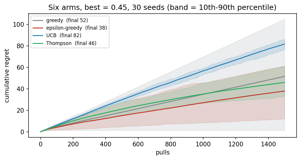
The experiment in detail. The four strategies are compared on a bandit with \(K = 6\) arms whose probabilities lie close together: 0.30, 0.35, 0.38, 0.40, 0.42 and 0.45. The best arm is the sixth, with \(\mu^* = 0.45\). One run consists of \(T = 1500\) pulls. At every pull the experiment does four things. It chooses an arm by the rule of the strategy. It draws the reward, 1 with the probability of that arm and 0 otherwise. It adds one to \(N_a\) and the reward to \(S_a\). It records the loss \(\mu^* - \mu_{a_t}\) of the pull. The cumulative regret after each pull is the running sum of these losses.
Each strategy is run thirty times. A run is identified by its seed, the number that starts the random number generator: The same seed always produces the same run, and the seeds 0 to 29 give thirty different runs. For the final regrets \(x_1, \ldots, x_n\) of the \(n = 30\) runs, the experiment reports the mean, written \(\bar{x}\) with a bar, the standard deviation (SD), the usual measure of spread, and the largest value, the worst seed:
The 10th and the 90th percentile, which bound the bands of the figure, are the values below which 10 and 90 percent of the runs fall.
In the run with seed 0, UCB first pulls every arm once, in order. Arms 2, 3 and 4 pay, and arms 1, 5 and 6 do not. The losses of these six pulls are \(0.15 + 0.10 + 0.07 + 0.05 + 0.03 + 0 = 0.40\), the regret so far.
Pull 7 is the first that uses the rule. Every arm has \(N_a = 1\), so every bonus is \(2 \sqrt{\ln 7 / 1} = 2.79\). The sums are \(1 + 2.79 = 3.79\) for the three arms that paid and \(0 + 2.79 = 2.79\) for the others. Among equal sums the first arm is taken, here arm 2, and this pull does not pay.
At pull 8, arm 2 has the estimate \(1 / 2 = 0.5\) and the smaller bonus \(2 \sqrt{\ln 8 / 2} = 2.04\), a sum of 2.54. Arms 3 and 4 have \(1 + 2 \sqrt{\ln 8 / 1} = 3.88\), and UCB pulls arm 3. With bonuses this large, UCB returns to every arm many times before the estimates decide.
Animation. Mean cumulative regret of three strategies over 1500 pulls and twenty seeds. Change \(\varepsilon\) and the constant \(c\) of the upper confidence bound (UCB) and watch the ranking.
| Strategy | Mean final regret | Standard deviation | Worst seed |
|---|---|---|---|
| Greedy | 51.5 | 50.0 | 223.5 |
| Epsilon-greedy, \(\varepsilon = 0.1\) | 37.9 | 27.1 | 138.1 |
| Upper confidence bound (UCB), \(c = 2\) | 81.7 | 3.9 | 87.8 |
| Thompson sampling | 45.9 | 11.3 | 72.2 |
The figure shows the mean cumulative regret of each strategy, with a band between the 10th and the 90th percentile of the thirty runs, and the table gives the regret after the last pull. For comparison, pulling arms purely at random loses \(0.45 - 0.383 = 0.067\) per pull on average, about 100 over 1500 pulls. Epsilon-greedy ends with the lowest mean regret, about 38, followed by Thompson sampling with 46, greedy with 52 and UCB with 82. Greedy varies most: In its best seed it finds the best arm at once and loses less than 1, and in its worst seed it locks onto a poor arm and loses 224. UCB with \(c = 2\) varies least, but on arms this close and with so few pulls its bonus buys more exploration than it repays. Its guarantee concerns the long run [2].
The constant \(c\) decides how much UCB explores. The same experiment with other values of \(c\) gives:
| Constant \(c\) | Mean final regret | Worst seed |
|---|---|---|
| 0.25 | 42.8 | 112.7 |
| 0.5 | 40.6 | 60.3 |
| 1 | 63.1 | 89.0 |
| 2 | 81.7 | 87.8 |
| 4 | 89.8 | 94.2 |
A small constant explores too little and behaves like greedy in its bad seeds. A large one explores for too long. Here \(c = 0.5\) is the best compromise, with a mean regret of 41 and a worst seed of only 60. A mean alone would hide such differences. For this reason the standard deviation and the worst seed are reported next to every mean.

Python code in the Colab notebook, Section 1. Open Section 1 of the Colab notebook and run it. The function run_bandit contains the four rules, each as one line of Python, and the cell prints the two tables and draws the figure shown here. Then change c=2.0 or eps=0.1 in the first line of the function and run the cell again to see the ranking change.
Check your understanding. Why can a purely greedy strategy end with a large regret?
Check your understanding. An arm has been pulled 4 times and has paid 3 times. At pull number \(t = 100\) and with \(c = 2\), what is its upper confidence bound?
Markov decision processes
In most problems an action also changes the situation. A Markov decision process, abbreviated MDP, describes such a problem with five ingredients [1]: a set of states, a set of actions, transition probabilities, rewards and a discount factor. The transition probability \(P(s' \mid s, a)\) is the probability that the next state is \(s'\) when the agent takes action \(a\) in state \(s\). The reward \(r(s, a, s')\) is the number that the agent receives for this step. The Markov property says that the next state depends only on the current state and action, not on the whole history:
The discount factor \(\gamma\), the Greek letter gamma, is a number between 0 and 1 that makes rewards count less the later they come. With it the return becomes a discounted sum:
A reward that arrives \(k\) steps later is multiplied by \(\gamma^k\). One run from a start state to an end state is called an episode.
An episode gives the rewards 2, 0 and 10 and then ends. With \(\gamma = 0.9\) the return is \(2 + 0.9 \times 0 + 0.9^2 \times 10 = 2 + 0 + 8.1 = 10.1\). With \(\gamma = 0.5\) the same rewards give \(2 + 0 + 0.25 \times 10 = 4.5\): The late reward counts much less. With \(\gamma = 1\) nothing is discounted, and the return is the plain sum, 12.
The project of the course, TokenWorld, is a Markov decision process of this kind: The agent writes a short sentence one word at a time and is rewarded at the end for its quality. It is a miniature of how a language model is trained with reinforcement learning on Day 4. A unit of text, here a word, is called a token. The vocabulary has four tokens: the, cat, sat and <eos>, the end-of-sentence token. The state is the sentence written so far, the action is the next token, and the transition is certain: The token is appended. An episode ends when the agent writes <eos> or when the sentence has four tokens. Only then does the reward arrive, computed by the rules of the table, and no reward is discounted, \(\gamma = 1\). TokenWorld has 161 states: the empty sentence and 4, 12, 36 and 108 sentences of one, two, three and four tokens. Of these, 121 are finished sentences.
| Property of the finished sentence | Reward |
|---|---|
It starts with the | \(+1.0\), otherwise \(-0.5\) |
cat appears exactly once | \(+1.5\) |
cat does not appear | \(-0.5\) |
cat appears more than once | \(-0.8\) for every repetition |
sat appears, and the first cat stands before it | \(+1.0\) |
| Each word, the end token not counted | \(-0.25\) |
| The sentence has no word at all | \(-1.0\) as the whole reward |
For example, the sentence the cat sat <eos> earns \(1.0 + 1.5 + 1.0 - 3 \times 0.25 = 2.75\), and the sentence cat cat <eos> earns \(-0.5 - 0.8 - 2 \times 0.25 = -1.8\).
The count can be followed step by step. After the first token there are 4 sentences, of which 3 are unfinished, because one of them is <eos> alone. Each unfinished sentence can be continued with 4 tokens. This gives \(3 \times 4 = 12\) sentences of two tokens, 9 of them unfinished, then \(9 \times 4 = 36\) of three tokens, 27 of them unfinished, and \(27 \times 4 = 108\) of four tokens. Together with the empty sentence these are \(1 + 4 + 12 + 36 + 108 = 161\) states. Finished are the \(1 + 3 + 9 = 13\) shorter sentences that end with <eos> and all 108 sentences of four tokens, in total 121.
Python code in the Colab notebook, Section 2. Open Section 2 of the Colab notebook and run it. The function score_sequence is the reward table above written as Python code, and the function step appends one token to the sentence. The second cell counts the 161 states and prints the five best and the three worst sentences with their rewards.
Check your understanding. What does the discount factor control?
Values and the Bellman equation
The value of a state is the return the agent can expect from it when following its policy. As a formula, with \(\mathbb{E}_{\pi}\) for the average over everything that can happen while the agent follows the policy \(\pi\):
Bellman observed that values satisfy a recursive relation: The value of a state equals the expected reward of the next step plus the discounted value of the state that follows [4]. For a given policy \(\pi\) this relation is the Bellman expectation equation:
The two sums average over the action that the policy chooses and over the next state that follows. For the best possible policy, whose values are written \(V^*\), the average over the actions is replaced by the best action, which gives the Bellman optimality equation:
The formula is read from the inside. For one action \(a\), every possible next state \(s'\) contributes its reward plus its discounted value, weighted by its probability. The sum over \(s'\) is therefore the expected outcome of the action, called its action value \(Q^*(s, a)\). The max over \(a\) then picks the best action, and the best policy \(\pi^*\) takes that action:
One application of the right-hand side to one state is called a backup. A state has two actions, every step costs 1, and \(\gamma = 0.9\). The action left leads with certainty to a state of value 4, so its value is \(-1 + 0.9 \times 4 = 2.6\). The action right leads with probability 0.7 to a state of value 10 and with probability 0.3 to a state of value \(-5\), so its value is \(0.7 \times (-1 + 0.9 \times 10) + 0.3 \times (-1 + 0.9 \times (-5)) = 0.7 \times 8 - 0.3 \times 5.5 = 3.95\).
The value of the state is the larger of the two, 3.95, and the best action is right.
When the transitions are known, the equation can be solved by repeating it until the values stop changing, which is value iteration, a form of dynamic programming. All values start at zero. One sweep visits every state and replaces its value by the backup computed from the current values:
The index \(k\) counts the sweeps. They stop when the largest change of a value in one sweep, \(\max_s |V_{k+1}(s) - V_k(s)|\), falls below a small tolerance. Policy iteration is a second method for the same task. It reaches the same values along another route: It computes the values of the current policy by repeating the expectation equation, switches every state to the action with the highest action value, and repeats both steps until the policy no longer changes.
A corridor has two cells, A and B, and a goal behind B. The action forward moves the agent one cell on with probability 0.8 and leaves it where it is with probability 0.2. Every step has a reward of \(-1\), except the step that reaches the goal, which has a reward of 0, and \(\gamma = 0.9\). The goal has the value 0, and both cells start with the value 0.
Sweep 1 uses the starting values. For B: \(0.8 \times (0 + 0.9 \times 0) + 0.2 \times (-1 + 0.9 \times 0) = -0.2\). For A: \(0.8 \times (-1 + 0.9 \times 0) + 0.2 \times (-1 + 0.9 \times 0) = -1\).
Sweep 2 uses the values of sweep 1. For B: \(0.8 \times 0 + 0.2 \times (-1 + 0.9 \times (-0.2)) = -0.236\). For A: \(0.8 \times (-1 + 0.9 \times (-0.2)) + 0.2 \times (-1 + 0.9 \times (-1)) = -0.944 - 0.380 = -1.324\).
The next sweeps give \(-1.408\), \(-1.428\) and \(-1.432\) for A and \(-0.242\) and \(-0.244\) for B, and the values settle at \(-1.434\) and \(-0.244\). The largest change of a sweep shrinks from 1 to 0.32, 0.08, 0.02 and 0.004, and the sweeps stop when it falls below the tolerance. A second action, wait, would have the value \(-1 + 0.9\, V(s)\), which is lower in every sweep, so the max chooses forward.
The Windy Cliff is a grid of 4 rows and 8 columns. The agent starts in the bottom left corner and has to reach the goal in the bottom right corner, and the cells between them are a cliff. The four actions are up, down, left and right. Every step has a reward of \(-1\), except the step that reaches the goal, which has a reward of 0. A step into the cliff has a reward of \(-100\) and puts the agent back at the start. The wind is described by the slip probability, 0.15 in this example: With this probability the wind replaces the chosen action by a push to the left or to the right, each with half of it, 0.075. The discount factor is 0.99. The optimal policy walks along the row next to the cliff, the shortest route: A sideways push cannot move the agent down into the cliff from that row. The wind changes the values and not the route. The value of the start falls from \(-7.7\) without wind to \(-17.9\) with a slip probability of 0.15, because at the start a push to the right ends in the cliff. Value iteration computes the values of all 32 cells with the update above and stops when no value changes by more than \(10^{-9}\), here after 26 sweeps. Policy iteration ends with the same values after 4 changes of the policy. Part C of the interactive lab asks for one discounted return and one Bellman backup, computed by hand as in the worked examples.
Without wind the shortest route has nine steps: one up, seven to the right and one down into the goal. The first eight have a reward of \(-1\) and the last one a reward of 0. The value of the start is their discounted sum, \(-(1 + 0.99 + 0.99^2 + \cdots + 0.99^7) = -7.73\).
With a slip probability of 0.15, the action up at the start has three outcomes. With probability 0.85 the agent moves up, to a cell whose value is \(-8.09\). With probability 0.075 the wind pushes it to the right, into the cliff: a reward of \(-100\) and a return to the start. With probability 0.075 the wind pushes it to the left, against the edge of the grid: a reward of \(-1\), and the agent stays at the start.
The Bellman equation of the start, with \(V\) for its own value, is therefore \(V = 0.85 \times (-1 + 0.99 \times (-8.09)) + 0.075 \times (-100 + 0.99\, V) + 0.075 \times (-1 + 0.99\, V)\). Collecting the terms gives \(V = -15.23 + 0.1485\, V\), and so \(V = -15.23 / 0.8515 = -17.89\). The risk of the cliff alone accounts for \(0.075 \times 100 / 0.8515 = 8.8\) of this value.
Animation. Value iteration on the Windy Cliff, sweep by sweep. Change the slip probability and run again: The arrows of the greedy policy keep their route, and the value of the start falls as the wind grows.
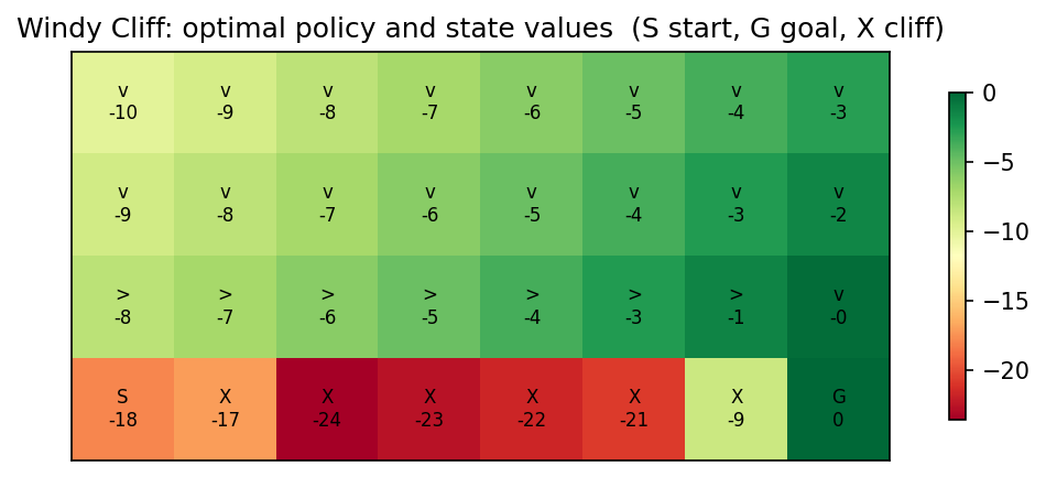
Python code in the Colab notebook, Section 3. Open Section 3 of the Colab notebook and run its cells. The function grid_transitions builds the transition probabilities, and the loop under the comment value iteration is the update above. The cells print the value of the start, \(-17.89\), and draw the figure shown here. Then change slip=0.15 to slip=0.0 where grid_transitions is called and run the cells again: The route stays, and the value of the start becomes \(-7.73\).
Check your understanding. With a slip probability of 0.15, the start of the Windy Cliff has a value of about minus 18 and the cell above it about minus 8. Why is the start so much worse?
An exact optimum as a yardstick
TokenWorld is small enough to be solved exactly, and this solution is the first result of the project. The best sentence is the cat sat <eos> with a return of 2.75, and value iteration finds the same number as the value of the empty sentence, the state in which every episode starts. The best policy writes this sentence token by token.
The table shows how the best policy decides. For the sentence written so far, each column gives the action value \(Q^*\) of writing that token next and continuing in the best way. The best policy takes the largest value of each row.
| Sentence so far | the | cat | sat | <eos> | Best next token |
|---|---|---|---|---|---|
| (empty) | \(2.75\) | \(1.50\) | \(0.50\) | \(-1.00\) | the |
the | \(2.50\) | \(2.75\) | \(1.75\) | \(0.25\) | cat |
the cat | \(2.50\) | \(0.20\) | \(2.75\) | \(2.00\) | sat |
the cat sat | \(2.50\) | \(0.20\) | \(2.50\) | \(2.75\) | <eos> |
The values are computed from the end of the sentence backwards. After the cat sat every action ends the episode, so each action value is the reward of the finished sentence. Writing <eos> gives \(1.0 + 1.5 + 1.0 - 3 \times 0.25 = 2.75\). Writing the or sat gives a sentence of four words with one cat, \(1.0 + 1.5 + 1.0 - 4 \times 0.25 = 2.50\). Writing cat gives the cat sat cat, in which cat is repeated: \(1.0 - 0.8 + 1.0 - 4 \times 0.25 = 0.20\). The value of the state the cat sat is the largest of these, 2.75.
One step earlier, after the cat, the action sat leads to that state, so its action value is 2.75. The action <eos> ends with the cat <eos>, which earns \(1.0 + 1.5 - 2 \times 0.25 = 2.00\). The other two actions lead to states whose values, 2.50 and 0.20, are found in the same way. The largest value is again 2.75, and the best token is sat.
A policy that picks each token at random, with probability \(1/4\), writes the best sentence with probability \((1/4)^4 = 1/256\), less than once in two hundred tries. Its expected return is the reward of every finished sentence \(x\), weighted by the probability of writing it:
Here \(|x|\) is the number of tokens of the sentence, the end token included, and \(R(x)\) is its reward.
The sum has 121 terms and can be followed by the length of the sentences. The single sentence of one token, <eos> alone, has the probability \(1/4\) and the reward \(-1\), a contribution of \(-0.250\). The 3 finished sentences of two tokens have the probability \(1/16\) each and rewards that add up to \(-0.25\), a contribution of \(-0.016\). The 9 of three tokens, with \(1/64\) each, contribute \(-0.005\). The 108 of four tokens, with \(1/256\) each and rewards that add up to \(-57.05\), contribute \(-0.223\). The total is \(-0.493\).
A simulation estimates the same number: 4000 episodes played with the random policy have a mean return of \(-0.526\). The difference from the exact value is due to chance. One random episode has a standard deviation of 1.20, so the mean of 4000 episodes is uncertain by about \(1.20 / \sqrt{4000} = 0.019\). This quantity, the standard deviation divided by the square root of the number of episodes, is called the standard error of the mean. Of the 4000 episodes, 0.35 percent reached the optimum, close to the exact share of \(1 / 256\), which is 0.39 percent.
Every learning method of the week is measured against the exact optimum of 2.75, which turns a vague claim that a method works into a number.
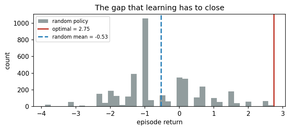
Python code in the Colab notebook, Section 4. Open Section 4 of the Colab notebook and run it. The function value_iteration_tokenworld computes the action values, and the cell prints the table above row by row. The next cell plays the 4000 random episodes, prints their mean return and draws the histogram shown here.
Your field
Bandits appear wherever options are tested on the fly: doses in a clinical trial, subject lines of an email campaign, tariffs offered to drivers, irrigation schedules or hint styles in a tutoring system. The application of the day poses such a problem for five fields. For medicine, the four arms are four doses to which a patient responds with the probabilities 0.20, 0.35, 0.50 and 0.45. The four strategies of the day run on these arms for 1000 pulls and over 20 seeds. Epsilon-greedy and Thompson sampling end with mean regrets of about 25 and 26, greedy with 58 and UCB with \(c = 2\) with 69.
Python code in the Colab notebook, Section 5. Open Section 5 of the Colab notebook. Its first line is a switch, FIELD = "medicine". Replace the word by marketing, energy, agriculture or education and run the section. The printed table shows which strategy has the lowest mean regret in that field and which has the smallest spread.
Going further (optional)
Results in reinforcement learning vary strongly from one random seed to the next, so a single run proves little [6]. The rest of the week therefore follows three habits: Every method is run over many seeds, the spread is reported next to the mean, and an estimate is checked against an exact value wherever one exists.
TokenWorld puts these habits to work. The best policy writes a random token with probability \(\varepsilon\), and each such policy is evaluated with 15 seeds of 400 episodes each:
| Share of random tokens \(\varepsilon\) | Mean return over 15 seeds | Standard deviation of the seeds |
|---|---|---|
| 0 | \(2.750\) | 0.000 |
| 0.1 | \(2.320\) | 0.035 |
| 0.3 | \(1.534\) | 0.050 |
| 0.6 | \(0.606\) | 0.053 |
| 1 | \(-0.478\) | 0.052 |
With \(\varepsilon = 1\) the policy is the random policy, whose exact expected return is \(-0.493\). The measured \(-0.478\) agrees with it within the uncertainty. One seed averages 400 episodes, so its mean varies from seed to seed by about \(1.20 / \sqrt{400} = 0.060\), close to the measured 0.052. The mean of 15 seeds is uncertain by about \(0.060 / \sqrt{15} = 0.016\), and the two numbers differ by 0.015.
Python code in the Colab notebook, Section 6. Open Section 6 of the Colab notebook and run it. The function study evaluates one policy over 15 seeds and returns the mean, the standard deviation and the best and the worst seed, and the cell prints the table above. The last cell shows three sliders, for \(\varepsilon\), for \(c\) and for the number of seeds: Move them and watch the regret curves of the bandit change.
Python step 1: Values, variables, lists and decisions
Python code in the Colab notebook, right after Section 0 (setup). Open the notebook and run this step cell by cell: It consists of short pieces of Python code with their explanations, a quick check and three exercises. Topics: Values, lists and variables · A decision: explore or exploit · A loop of 300 pulls · A function for the regret · A dictionary of results.
Students who have never programmed start with the start-here notebook of the course.
The notebook continues with the hands-on sections, and the interactive lab holds three practice parts and the self-assessment. The study path, the daily task and the research assignment are on the day overview.
Review cards
Select a card to turn it over.
References
[1] Sutton, R. S., & Barto, A. G. (2018). Reinforcement Learning: An Introduction (2nd ed.). MIT Press.
[2] Auer, P., Cesa-Bianchi, N., & Fischer, P. (2002). Finite-time analysis of the multiarmed bandit problem. Machine Learning, 47(2-3), 235-256.
[3] Thompson, W. R. (1933). On the likelihood that one unknown probability exceeds another in view of the evidence of two samples. Biometrika, 25(3-4), 285-294.
[4] Bellman, R. (1957). A Markovian decision process. Journal of Mathematics and Mechanics, 6(5), 679-684.
[5] Van Rossum, G., & Drake, F. L. (2009). Python 3 Reference Manual. CreateSpace.
[6] Henderson, P., Islam, R., Bachman, P., Pineau, J., Precup, D., & Meger, D. (2018). Deep reinforcement learning that matters. In Proceedings of the AAAI Conference on Artificial Intelligence, 32(1), 3207-3214.
[7] Kluyver, T., Ragan-Kelley, B., Pérez, F., Granger, B., Bussonnier, M., Frederic, J., Kelley, K., Hamrick, J., Grout, J., Corlay, S., et al. (2016). Jupyter Notebooks: A publishing format for reproducible computational workflows. In Positioning and Power in Academic Publishing: Players, Agents and Agendas (pp. 87-90). IOS Press.