Overview
Day 1 solved problems whose transitions were known. In practice an agent rarely has such a model; it must learn from its own experience. This day covers the methods that learn values directly from experience: Monte Carlo methods, which wait for the end of an episode, temporal difference learning, which learns from each step [1], and two control methods. These are SARSA, named after the state, action, reward, state and action that one of its updates uses [2], and Q-learning [3], and they differ in one detail with large consequences near a cliff. The day ends with a deep Q-network, whose two engineering ideas, replay and a target network [4, 5], are tested by removing them.
Day at a glance
flowchart LR
  A["Learning without a model"] --> B["Monte Carlo and temporal differences"]
  B --> C["SARSA and Q-learning"]
  C --> D["The cliff"]
  D --> E["Deep Q-networks"]
  E --> F["Your field"]
  F --> G["Python step 2"]
Every method on this page is also written as Python code in the Colab notebook of the day. A Colab notebook is a document of text and Python code that runs in the web browser, with nothing to install. Its code is divided into numbered sections. Each orange box on this page names the section whose code carries out what the text above the box explains. The box says what to run and what to look at in that section, and its button opens the notebook at that place. The practice parts and the self-assessment of the day are in the interactive lab.
Learning without a model
Day 1 described TokenWorld, the project of the course, as a Markov decision process: An agent writes a sentence of at most four tokens from the vocabulary the, cat, sat and <eos>, the end-of-sentence token, and the finished sentence earns a reward by fixed rules. Because the rules were known, value iteration solved TokenWorld exactly. The best sentence, the cat sat <eos>, earns 2.75, and a policy that writes at random earns \(-0.49\) on average.
This day takes the rules away. The agent no longer knows where a token leads or what a sentence will earn: It can only write sentences and observe their rewards. The day measures how close methods that learn from such experience come to the optimum of Day 1, which remains the scoreboard of every experiment. Its last part replaces the table of values by a neural network, the first step towards the language model of Day 4.
Day 1 described a decision problem as a Markov decision process, abbreviated MDP: states, actions, transition probabilities, rewards and a discount factor. The transition probabilities and the rewards together are called the model of the environment. Value iteration needs the model, because each of its updates sums over all possible next states. Methods that compute values from a model are called dynamic programming. A learning agent has no model: It can only act and observe, and its experience is a stream of states, actions, rewards and next states. Without a model, values are estimated from experience.
The symbols are those of Day 1. At step \(t\) the agent is in the state \(s_t\), takes the action \(a_t\) and receives the reward \(r_{t+1}\) and the next state \(s_{t+1}\). Its policy \(\pi(a \mid s)\), with the Greek letter pi, is the probability of taking action \(a\) in state \(s\). An episode is one run from the start to an end state, also called a terminal state. The return \(G_t\) adds up the rewards after step \(t\), each multiplied by a power of the discount factor \(\gamma\), the Greek letter gamma. The value of a state is the return that the agent can expect from it under its policy:
The sign \(\mathbb{E}_{\pi}\) is the average over everything that can happen while the agent follows \(\pi\), and the vertical bar reads given. Finding \(V^{\pi}\) for a given policy is called policy evaluation. The agent keeps a table with one estimate per state. An estimate is marked with a hat: \(\hat{V}(s)\) is the number in the table, and \(V^{\pi}(s)\) is the exact value that it should approach. A method that produces such estimates from data is called an estimator.
Every method of this day changes an estimate in the same way. It computes a target, a number that the estimate should come closer to, and moves the estimate a part of the way towards it:
The number \(\alpha\), the Greek letter alpha, lies between 0 and 1 and is called the step size or learning rate. With \(\alpha = 0.1\) the estimate moves one tenth of the way to the target. The methods of the day differ in the target.
Monte Carlo. A Monte Carlo method plays an episode to its end and moves the value of each visited state towards the return that actually followed. Its target is the return \(G_t\):
The arrow reads is replaced by. The update is made for every state of the episode, after the episode has ended, because \(G_t\) is not known earlier. The name Monte Carlo stands for methods that estimate an average from random samples, here from complete episodes.
Temporal differences. A temporal difference (TD) method does not wait: After each step it moves the value of the state towards the reward plus the discounted value of the next state, an estimate built on another estimate [1]. The difference between this target and the old estimate is written \(\delta_t\), with the Greek letter delta:
The target is \(r_{t+1} + \gamma \hat{V}(s_{t+1})\), and \(\delta_t\) is called the temporal difference error or TD error. When \(s_{t+1}\) is terminal, nothing follows it, and the target is the reward alone. Building an estimate on another estimate is called bootstrapping. The figures label this method TD(0): The zero says that the target looks one step ahead before it bootstraps.
The TD target rests on the Bellman equation of a policy [8]: The value of a state is the expected reward of the next step plus the discounted value of the state that follows.
Here \(P(s' \mid s, a)\) is the probability that action \(a\) in state \(s\) leads to the next state \(s'\), and \(r(s, a, s')\) is the reward of that step. The two sums, written with the sign \(\sum\), average over the action that the policy chooses and over the state that follows. With a model, the right-hand side can be computed, which is how the exact values that score the estimates of this day are obtained. Without a model, one step of experience gives one sample of the bracket, with \(\hat{V}\) in place of the unknown \(V^{\pi}\), and TD takes this sample as its target.
Monte Carlo is unbiased but noisy; TD is less noisy but starts from biased guesses. Unbiased means right on average: The mean of many returns from a state is its value. Noisy means that a single return can lie far from this mean, because it depends on every random choice until the end of the episode. A TD target depends on one step and varies less, but it contains the estimate of the next state, which is wrong at the beginning. This systematic error is called bias.
All estimates are zero, \(\alpha = 0.05\) and \(\gamma = 1\). The agent writes the sentence the cat sat <eos> of TokenWorld. Its first three steps have a reward of 0 and the last step a reward of 2.75, so the return from each of the four visited states is 2.75.
Monte Carlo moves all four estimates to \(0 + 0.05 \times (2.75 - 0) = 0.1375\). TD changes only the last state: Its target is the reward 2.75, and its estimate becomes 0.1375. For the three earlier states the target is \(0 + \hat{V}(s_{t+1}) = 0\), so the TD error is zero and nothing changes.
After a second episode with the same sentence, Monte Carlo holds \(0.1375 + 0.05 \times (2.75 - 0.1375) = 0.268\) for all four states. TD holds 0.268 for the last state, \(0.05 \times 0.1375 = 0.007\) for the state before it and still zero for the first two: The final reward travels back by one state per episode.
In the project, the two estimators evaluate one policy of TokenWorld. The state is the sentence written so far, called a prefix while it is unfinished, and the action is the next token. An episode ends with <eos> or with the fourth token. Every reward is zero except the last one, which scores the finished sentence by the rules of the reward table of Day 1, and nothing is discounted, \(\gamma = 1\). TokenWorld has 161 states, of which 40 are prefixes: the empty sentence and 3, 9 and 27 prefixes of one, two and three words.
The best sentence, the cat sat <eos>, starts with the, contains cat once and has sat after it, and each of its three words costs 0.25: It earns \(1.0 + 1.5 + 1.0 - 3 \times 0.25 = 2.75\). This exact optimum of Day 1 is the scoreboard of the day.
The policy that produces the episodes, the behaviour policy, writes the best next token with probability 0.7375 and each other token with probability 0.0875. Its exact value at the empty sentence is 1.38. Both estimators learn from the same 3000 episodes with \(\alpha = 0.05\), and the experiment is repeated with ten seeds. A seed is the number that starts the random number generator, so ten seeds give ten different runs. A table of estimates is scored by its root mean square error, abbreviated RMSE, over the \(n = 40\) prefixes:
Each error is squared, the squares are averaged, and the root brings the result back to the unit of the values. A table of zeros, the start of both methods, has an RMSE of 1.25.
The exact values come from the Bellman equation of the policy, applied from the end of the sentence backwards. After the cat sat every token ends the episode. The best token <eos> is written with probability 0.7375 and earns 2.75. The tokens the, cat and sat are written with probability 0.0875 each and earn 2.50, 0.20 and 2.50. The value of this prefix is \(0.7375 \times 2.75 + 0.0875 \times (2.50 + 0.20 + 2.50) = 2.028 + 0.455 = 2.483\).
One step earlier, after the cat, the best token sat leads to that prefix. The token <eos> ends the sentence with a reward of 2.00, and the tokens the and cat lead to prefixes whose values, 2.058 and \(-0.111\), are found in the same way. The value is \(0.7375 \times 2.483 + 0.0875 \times (2.058 - 0.111 + 2.00) = 2.177\).
The same step gives 1.886 for the prefix the and, at the empty sentence, \(0.7375 \times 1.886 + 0.0875 \times (0.870 - 0.021 - 1.00) = 1.391 - 0.013 = 1.378\). The policy earns 1.38 on average, half of the optimum of 2.75, because every exploring token can spoil the sentence.
After 100, 500 and 3000 episodes the mean error of Monte Carlo is 0.99, 0.81 and 0.59, and that of TD is 1.05, 0.85 and 0.61. Monte Carlo is ahead in each of the ten seeds. The figure that this code draws shows both error curves with a band from the 10th to the 90th percentile, the values below which 10 and 90 percent of the seeds fall. Two facts explain the result. The single reward comes at the end, so TD has to wait until it has travelled back through the prefixes, as in the worked example. And the behaviour policy writes 26 of the 40 prefixes in fewer than one episode out of a hundred. Their estimates stay close to zero and carry most of the error, and a TD target built on such a prefix inherits its error. On the 14 prefixes that are written often, the two methods are almost equally accurate, with errors of about 0.13 and 0.12.
The opposite case is the random walk of the animation. Five states in a row are named A to E, and every episode starts in the middle state C. At each step the agent moves one state to the left or to the right, each with probability one half, so there is no choice and the policy is fixed. The episode ends when the agent leaves the row. Leaving on the right, beyond E, gives a reward of 1, every other step a reward of 0, and nothing is discounted. The value of a state is therefore the probability of leaving on the right: \(1/6\), \(2/6\), \(3/6\), \(4/6\) and \(5/6\) for A to E. An episode lasts 9 steps on average, and its return is 0 or 1 like the toss of a coin. Both tables start at 0.5 for every state.
Animation. Monte Carlo and temporal difference (TD) learning on the five-state random walk, averaged over 40 runs. The lines show the mean estimates next to the true values, and the readout shows the root mean square error (RMSE) of each method. Change the step size and the number of episodes and compare the errors.
With the default step size of 0.1 and 100 episodes, the readout shows an RMSE of 0.160 for Monte Carlo and 0.052 for TD. A return of 0 or 1 is a noisy target for a state whose value is one half, and with a constant step size this noise never averages out. The TD target of the middle state is the estimate of a neighbour, close to \(1/3\) or \(2/3\), and varies three times less. The bias of TD shows at the smallest step size, 0.01. After 100 episodes its estimates for B and D are 0.45 and 0.55, still close to the starting value, and Monte Carlo is ahead with 0.096 against 0.128.
Which one learns faster depends on the problem: On TokenWorld, whose reward comes only at the end, Monte Carlo wins; on a random walk with many steps, TD wins. The structure of a problem suggests the winner. Long episodes with many random steps make returns noisy and favour TD. A single reward at the end of a short episode and many rarely visited states favour Monte Carlo, because TD waits for the reward to travel back and builds its targets on poor estimates. A measurement against exact values decides.

Python code in the Colab notebook, Section 2. Open Section 2 of the Colab notebook and run it. The function behaviour_policy defines the policy that is evaluated, the loop under the comment ground truth computes its exact values, and the function evaluate_mc_td contains the two updates of this section. The cell prints the error of both methods after 100, 500 and 3000 episodes and draws the two error curves.
Check your understanding. What does a temporal difference update use instead of the full return?
Check your understanding. A state has the estimate 0.40. One step gives a reward of 0 and leads to a state with the estimate 0.90. With \(\gamma = 1\) and \(\alpha = 0.1\), what is the estimate of the first state after a TD update?
SARSA and Q-learning
Evaluating a given policy is one half of the problem. The other half, finding a good policy, is called control. To improve behaviour, the agent learns the values of actions, Q-values, and prefers actions with high values while still exploring. The action value \(Q^{\pi}(s, a)\) is the return that the agent can expect when it takes action \(a\) in state \(s\) and follows the policy \(\pi\) afterwards:
State values are not enough without a model: To choose between actions with \(V\), the agent would have to know where each action leads. A Q-table holds one estimate \(\hat{Q}(s, a)\) for every pair of a state and an action, and the action with the largest entry in the current state is called the greedy action. The action values of the best possible policy are written \(Q^*(s, a)\).
An agent that always takes the greedy action never tries the others and cannot discover that one of them is better. The epsilon-greedy rule of Day 1, written \(\varepsilon\)-greedy with the Greek letter epsilon, therefore explores with a small probability:
The symbol arg max returns the action with the largest entry. With \(K\) actions, the random choice falls on each of them with probability \(\varepsilon / K\), the greedy one included. The greedy action is therefore taken with probability \(1 - \varepsilon + \varepsilon / K\). With \(\varepsilon = 0.2\) and the four tokens of TokenWorld this is 0.85, and 0.05 remains for each other token. The behaviour policy of the comparison above is the same rule with \(\varepsilon = 0.35\) around the best tokens: \(0.65 + 0.35 / 4 = 0.7375\).
Both control methods of the day apply the TD update to Q-values. The agent takes the action \(a_t\) in the state \(s_t\), receives \(r_{t+1}\) and \(s_{t+1}\), and chooses its next action \(a_{t+1}\) with the \(\varepsilon\)-greedy rule. SARSA updates towards the value of the action it will actually take next, including exploratory ones [2]:
The name SARSA lists the five items of one update: state, action, reward, next state and next action. Q-learning updates towards the value of the best next action, whatever it actually does [3]:
Here \(\max_{a'}\) takes the largest entry of the next state over all actions \(a'\). In both rules the bracket is a TD error, and when \(s_{t+1}\) is terminal the target is the reward alone.
The policy that chooses the actions during learning is called the behaviour policy, and the policy whose values are learned is the target policy. SARSA learns about the policy it follows and is called on-policy. Q-learning learns about the greedy policy while exploring and is called off-policy. The difference between the two methods comes from exploration alone: When the next action is the greedy one, the two targets are the same number, and with \(\varepsilon = 0\) the two methods would be one. On TokenWorld with \(\varepsilon = 0.2\), for example, the first token the is worth 2.75 under the greedy policy and about 2.25 under the policy that keeps exploring.
The entry of the current state and action is \(\hat{Q}(s, a) = 1.2\), the step has a reward of 0, \(\alpha = 0.1\) and \(\gamma = 1\). In the next state the largest entry is 2.0, but the agent explores and chooses an action whose entry is 0.5.
Q-learning uses the largest entry: The target is \(0 + 2.0 = 2.0\), and the new value is \(1.2 + 0.1 \times (2.0 - 1.2) = 1.28\). SARSA uses the chosen action: The target is \(0 + 0.5 = 0.5\), and the new value is \(1.2 + 0.1 \times (0.5 - 1.2) = 1.13\). Had the agent chosen the greedy action, both methods would have written 1.28.
The whole algorithm is short. All entries start at zero. At the start of an episode the agent chooses an action with the \(\varepsilon\)-greedy rule. Then it repeats four things until the next state is terminal: It takes the action, observes the reward and the next state, chooses the next action, and applies the update. In the project, both methods learn TokenWorld for 4000 episodes with \(\alpha = 0.1\), \(\varepsilon = 0.2\) and \(\gamma = 1\), over ten seeds. The table has 160 entries, four tokens for each of the 40 prefixes.
Two numbers score a learned table, and both use the exact solution of Day 1. The first is the return of the greedy policy: the reward of the sentence that results when the greedy token is taken at every prefix, at best 2.75. The second is the RMSE of the 160 entries against the optimal action values \(Q^*(s, a)\). After 4000 episodes the greedy policy of Q-learning earns 2.25 on average, 82 percent of the optimum, and that of SARSA 2.55, 93 percent. The errors of the values are 1.23 and 1.22, where a table of zeros has 1.54.
Neither method has finished learning. Q-learning writes the best sentence in 2 of the 10 seeds and SARSA in 4, and most other runs have settled on a sentence that earns 2.5, such as the cat the sat. The large error has a plain cause: With a constant \(\varepsilon\) of 0.2 the agent mostly repeats its current sentence. In a run of Q-learning about 50 of the 160 pairs are never tried and keep their starting value of zero, and on the pairs tried at least 50 times the error is about 0.4. The last section of this lecture, Going further, gives schedules for \(\varepsilon\) and \(\alpha\) that bring Q-learning to the optimum in every seed. Part C of the interactive lab computes one update of each by hand.
Python code in the Colab notebook, Section 3. Open Section 3 of the Colab notebook and run it. The functions greedy_return and q_rmse compute the two scores. The function tabular_control trains either method, and its variable boot is the only line in which they differ: the entry of the action chosen next for SARSA, the largest entry of the next state for Q-learning. The cell prints the return of the greedy policy and the RMSE of each method and draws both scores over the 4000 episodes.
Check your understanding. Q-learning updates towards the best next action even when the agent explores. What is this property called?
The cliff
The difference shows on a cliff, the grid of the Windy Cliff of Day 1, with 4 rows and 8 columns. The start is the bottom left corner, the goal is the bottom right corner, and the six cells between them are the cliff. The actions are up, down, left and right, and a move against the border leaves the agent in its cell. Every step has a reward of \(-1\), except the step that reaches the goal, which has a reward of 0 and ends the episode. A step into the cliff has a reward of \(-100\) and puts the agent back at the start. In this section the wind of Day 1 is switched off and nothing is discounted, \(\gamma = 1\), so the only source of risk is the agent's own exploration.
Two routes matter. The shortest one goes up one cell, runs along the row above the cliff and comes down at the goal: 9 steps and a return of \(-8\). A longer one climbs to the top row and needs 13 steps, a return of \(-12\). Q-learning learns the shortest path along the edge, which would be optimal if the agent never explored; while it still explores, it sometimes steps off. SARSA takes its own exploration into account and learns a path further from the edge.
Both methods run for 800 episodes with \(\alpha = 0.5\) and \(\varepsilon = 0.1\), an episode is cut off after 300 steps, and ten seeds are used. Two measures describe the result. The greedy path is the path that results when the agent takes the greedy action of the learned table in every cell. The online return is the return of an episode as it was played during learning, exploring steps and falls included, averaged over the last 100 episodes. In every seed the greedy path of Q-learning is the 9-step path along the edge, and that of SARSA is a 13-step path through the top row. The online return is \(-31.0\) for Q-learning and \(-19.1\) for SARSA. During learning, SARSA therefore collects clearly more reward, although Q-learning's final greedy path is shorter.
On the path along the edge, seven cells have the cliff as a neighbour: the start and the six cells above the cliff. In each of them an exploring step ends in the cliff when the random action points at it. With \(\varepsilon = 0.1\) and four actions this happens with probability \(0.1 / 4 = 0.025\) per step.
The probability of passing all seven cells without a fall is \(0.975^7 = 0.84\). About 16 percent of the walks along the edge therefore end in the cliff, at a cost of 100, and start again. An exact evaluation of this exploring policy with the Bellman equation gives an expected return of about \(-31\) per episode. This is the online return measured for Q-learning, although the same path earns \(-8\) without exploration. On the 13-step path only the start has the cliff as a neighbour.
Animation. Greedy paths of Q-learning and SARSA after 500 episodes on the cliff without wind, with their online returns, averaged over the last 100 episodes. Raise the exploration rate \(\varepsilon\) and compare the two returns.
The animation repeats the experiment in the browser with one seed and 500 episodes. At the default \(\varepsilon = 0.1\) it shows \(-28.0\) for Q-learning and \(-21.4\) for SARSA. Q-learning keeps the path along the edge at every setting, and its online return falls from about \(-10\) at \(\varepsilon = 0.01\) to about \(-118\) at \(\varepsilon = 0.3\), where SARSA stands at about \(-44\). From 0.02 to 0.05, Q-learning has the better online return: Falls are then so rare that the four extra steps of the detour cost more. The path of SARSA changes from setting to setting and at some settings does not reach the goal, because one run of 500 episodes leaves its table unfinished.
Which is better depends on whether mistakes during learning are expensive, as they are for a real robot. When exploration stops after training, the shorter path of Q-learning is the better result. When the agent keeps exploring while it is in use, the values of SARSA describe what will really happen.
Python code in the Colab notebook, Section 4. Open Section 4 of the Colab notebook and run it. The function cliff_control is the code of Section 3 moved to the grid, and its option slip=0.0 switches the wind off. The cell prints, for each method, the number of steps of its greedy path and its online return over the last 100 episodes.
Check your understanding. Why does SARSA collect more reward than Q-learning while learning on the cliff?
Check your understanding. An agent explores with \(\varepsilon = 0.2\) and stands in a cell above the cliff. Its greedy action points along the edge. How likely is it that its next step ends in the cliff?
Deep Q-networks
A table needs one entry for every pair of a state and an action. TokenWorld has 160 pairs, but a language model that writes long texts from thousands of tokens has more states than any memory can hold. When states are too many for a table, a neural network approximates the Q-values. Computing values from a set of adjustable numbers, called weights, is called function approximation. Learning then means changing the weights, and one change moves the values of many states at once. On TokenWorld a table would still do. The network is trained there all the same, because the exact \(Q^*\) of Day 1 is known and the error of the network can be measured.
The network. A neural network is a function built from layers of simple operations. The network of this code first writes the state as a list \(x\) of 20 numbers. Each of the four positions of the sentence holds one of the four tokens or is still empty, and gets five numbers: a 1 for its content and 0 elsewhere. This is called a one-hot encoding. Two layers follow:
The first layer multiplies \(x\) by the matrix \(W_1\), adds the vector \(b_1\) and replaces every negative result by zero, an operation called rectified linear unit and abbreviated ReLU. Its 64 results form the hidden layer \(h\). The second layer turns \(h\) into four numbers, the Q-values of the four tokens, and the dot in \(\hat{Q}_w(s, \cdot)\) stands for all four actions at once. The letter \(w\) collects all weights, the entries of \(W_1\), \(b_1\), \(W_2\) and \(b_2\): \(20 \times 64 + 64 + 64 \times 4 + 4 = 1604\) numbers.
The target and the loss. The network is trained with the idea of Q-learning. A transition is the record of one step: the state \(s\), the action \(a\), the reward \(r\) and the next state \(s'\). Its target is
The weights \(w^-\) belong to the target network, which is explained below, and \(\gamma = 1\) on TokenWorld. The error on the transition is \(e = \hat{Q}_w(s, a) - y\), the output of the network minus the target. Training makes a loss small, a number that measures how wrong the network is. The loss used here is the Huber loss:
For errors up to 1 in size, the Huber loss is half the squared error. For larger errors it grows only in proportion to the error, so one wild target cannot pull the weights far. The loss of a batch of transitions is the mean of their losses.
A stored transition has a reward of 0 and a next state that is not terminal. The target network gives the four values 1.2, 2.4, 0.3 and 2.0 for the next state, so the target is \(y = 0 + 2.4 = 2.4\). The network gives 0.9 for the stored state and action. The error is \(e = 0.9 - 2.4 = -1.5\), larger than 1 in size, so the Huber loss is \(1.5 - 0.5 = 1.0\), where half the squared error would be \(1.5^2 / 2 = 1.125\).
A second transition ends its episode with a reward of 2.75, so its target is \(y = 2.75\). The network gives 2.5, the error is \(-0.25\), and the loss is \(0.25^2 / 2 = 0.031\).
The gradient. Training needs to know how the loss changes with every weight. This slope is found layer by layer, from the output back to the input, a procedure called backpropagation. For one transition, let \(d\) be a list of four numbers that is zero except at the action \(a\) that was taken. There it holds the slope of the Huber loss, which is the error \(e\) limited to the range from \(-1\) to 1. Then
The sign \(\partial\) marks a slope with respect to one group of weights. The product \(d\, h^{\top}\) is a table with one row per action and one column per hidden unit: Only the row of the action taken is not zero, and it holds \(h\) times the limited error. The list \(u\) carries the error back to the hidden layer. The sign \(\odot\) multiplies entry by entry, and \(\mathbf{1}[h > 0]\) is 1 where a hidden unit is active and 0 where the ReLU has set it to zero, so inactive units pass nothing back. The gradient \(g\) of a batch is the mean of these slopes over its transitions.
The update. The weights are changed by gradient descent. The gradient \(g\) holds for every weight the slope of the loss: the amount by which the loss grows when this weight grows a little. A step against the gradient, \(w \leftarrow w - \alpha g\), makes the loss smaller, with a learning rate \(\alpha\). The experiment uses a refined form of this step, the Adam optimiser, short for adaptive moment estimation. For every weight, Adam keeps a running average \(m\) of its gradient and a running average \(v\) of its squared gradient:
The index \(k\) counts the updates. The experiment uses \(\beta_1 = 0.9\) and \(\beta_2 = 0.999\), with the Greek letter beta, and \(\alpha = 0.003\). The divisions by \(1 - \beta_1^k\) and \(1 - \beta_2^k\) correct the two averages, which start at zero. Dividing by the root of \(v\) gives every weight a step of similar size, and the tiny number \(10^{-8}\) prevents a division by zero.
Two remedies. Training the network naively, on every step as it comes, is unstable: Successive samples are strongly correlated, and the target moves with every update. Correlated means that the steps of one episode resemble each other, so the network sees nearly the same input several times in a row. The target moves because it is computed by the network that is being changed. A deep Q-network, abbreviated DQN, adds two remedies [4]. Experience replay stores past transitions and trains on random batches of them [5], and a target network, a copy updated only now and then, keeps the target still.
In the experiment the store, called the replay buffer, has room for 4000 transitions, more than the at most 2800 steps of a run. As soon as it holds 64 transitions, every step of the agent is followed by one Adam update on a batch of 64 transitions drawn from it at random. A transition is therefore used about 60 times. The target network receives a fresh copy of the weights every 100 steps. The agent acts \(\varepsilon\)-greedily on the Q-values of the network, and \(\varepsilon\) falls in a straight line from 0.6 to 0.05:
Here \(i\) is the number of the episode, counted from 0, in a run of 700 episodes. Much exploration at the beginning fills the buffer with many different sentences.
What each part buys. The experiment removes each remedy in turn. An experiment that removes one part of a method to measure what it contributes is called an ablation. Each of the four configurations runs with three seeds, and the table shows the means of the two scores of the previous section.
| Configuration | Return of the greedy policy | Share of the optimum | RMSE of the Q-values |
|---|---|---|---|
| full DQN | 2.75 | 100 percent | 0.35 |
| without replay | 1.83 | 67 percent | 1.47 |
| without the target network | 2.75 | 100 percent | 0.58 |
| without both | 1.83 | 67 percent | 1.39 |
Without replay the network is trained on the latest transition alone, and none of its three runs reaches the optimum. Their greedy sentences earn 1.5, 1.5 and 2.5, on average two thirds of the optimum. Without the target network all three runs still write the best sentence, while the value estimates are clearly worse: The error rises from 0.35 to 0.58.
The third row shows that a greedy policy can be correct while the values behind it are wrong. The greedy action depends only on which entry of a state is the largest, and an error that leaves this order intact does not change the sentence. It does mislead every method that uses the values themselves, such as the actor-critic methods of Day 3.
The full network is also more accurate than the Q-table that Q-learning filled on TokenWorld, which ended with an error of 1.23 after 4000 episodes. It uses every transition many times, and its shared weights give values to pairs that were never tried. A run leaves about 40 of the 160 pairs untried. On them the error of the network is about 0.6, where the zeros of a table are off by about 1.7.
The max in the target has a known weakness. Among several uncertain estimates the largest one is more often too high than too low, so the targets are too high on average. Double Q-learning reduces this bias with the two sets of weights that a DQN already has [9]: The network chooses the best next action, and the target network evaluates it.
The application challenge for computer science asks for this target.
Python code in the Colab notebook, Section 5. Open Section 5 of the Colab notebook and run it. The class QNet is the network: Its function forward computes the Q-values, and train_step computes the gradient and makes the Adam update. The function dqn contains the replay buffer and the target network, and its options replay=False and target_net=False remove them. The cell prints the table of the four configurations.
Check your understanding. What does experience replay do?
Your field
The application of the day builds a gridworld from one of three fields: a warehouse with shelves and a forklift lane, a drone route with wind and a no-fly zone, or a building to evacuate with fire. SARSA and Q-learning learn in it side by side, and their greedy paths are drawn on the map. A gridworld is a world of cells like the cliff. Each domain has a start, a goal, walls and hazards. A move into a wall or across the border leaves the agent in its cell. A step into a hazard has the penalty of the domain as its reward and puts the agent back at the start. Every other step has a reward of \(-1\), and the step that reaches the goal a reward of 0. With the slip probability of the domain, the chosen action is replaced by a random one of the four.
| Domain | Grid | Walls | Hazards | Slip probability | Penalty |
|---|---|---|---|---|---|
| warehouse | 6 rows, 8 columns | 7 cells of shelves | 3 cells of a forklift lane | 0.05 | \(-20\) |
| drone | 5 rows, 8 columns | 2 cells | 6 cells of a no-fly zone in the bottom row | 0.20 | \(-50\) |
| evacuation | 6 rows, 6 columns | 5 cells | 3 cells of fire and smoke | 0.10 | \(-100\) |
Both methods run for 800 episodes with \(\alpha = 0.2\), \(\gamma = 0.98\) and \(\varepsilon = 0.1\), an episode is cut off after 200 steps, and five seeds are used. Each method is judged by its mean online return over the last 200 episodes and by the worst of these episodes. In the warehouse the two methods end level, with \(-13.4\) for SARSA and \(-13.5\) for Q-learning. Both greedy paths need 12 steps and pass no cell next to the forklift lane, so a single exploring step cannot lead into a hazard.
A slip belongs to the environment and not to the policy, so its cost enters the targets of both methods. In the drone domain, where one move in five slips, both greedy paths of the first seed fly one row above the direct route, which runs right over the no-fly zone. They need 9 steps where 7 would do. Which method collects more reward while learning differs from domain to domain.
Python code in the Colab notebook, Section 6. Open Section 6 of the Colab notebook. Its first line is a switch, DOMAIN = "warehouse". Replace the word by drone or evacuation and run the section. The function td_control trains SARSA and Q-learning on the map of that field, and the cell prints their online returns and draws the two greedy paths on the map.
Going further (optional)
Two topics deepen the day. The first is the choice of schedules for the exploration rate and the step size. The second is the deadly triad, a combination of three techniques under which learning can fall apart.
Schedules. A schedule is a rule that changes a setting during learning. The Q-learning experiment on TokenWorld is repeated with three schedules for the exploration rate, called const, decay and 1/t. Here \(i\) is the number of the episode, counted from 0, in a run of 4000 episodes:
The decay schedule falls in a straight line from 0.5 and is held at 0.02 during the last 160 episodes. The 1/t schedule starts at 1, has fallen to 0.5 after 200 episodes and ends near 0.05. They are combined with three schedules for the step size, in which \(N(s, a)\) counts the updates that the pair of state and action has received, the current one included:
With the step size \(1 / N(s, a)\) the estimate is exactly the mean of all targets that the pair has received. The schedule poly, short for polynomial, shrinks more slowly, so later targets count more. This suits Q-learning, whose targets improve while the later prefixes are being learned.
At episode 1000 the decay schedule gives \(\varepsilon = 0.5 \times (1 - 1000 / 4000) = 0.375\), and the 1/t schedule gives \(1 / (1 + 5) = 0.167\).
A pair that receives its tenth update has the step size \(1 / 10 = 0.1\) under 1/n and \(10^{-0.7} = 0.20\) under poly. At the hundredth update the step sizes are 0.01 and 0.04: Under poly a new target still counts four times as much.
| Exploration | Step size | Mean return of the greedy policy | Seeds at the optimum | RMSE of the Q-values |
|---|---|---|---|---|
| decay | poly | 2.75 | 8 of 8 | 0.52 |
| decay | 1/n | 2.72 | 7 of 8 | 0.57 |
| 1/t | poly | 2.75 | 8 of 8 | 0.76 |
| 1/t | 1/n | 2.56 | 6 of 8 | 0.77 |
| const | poly | 2.72 | 7 of 8 | 0.90 |
| const | 1/n | 2.66 | 5 of 8 | 0.96 |
| decay | const | 2.63 | 6 of 8 | 1.08 |
| const | const | 2.28 | 1 of 8 | 1.23 |
| 1/t | const | 1.78 | 1 of 8 | 1.23 |
The table lists the nine combinations after 4000 episodes and eight seeds, sorted by the error of the values. The schedules of the exploration rate and the step size decide whether a method reaches the optimum at all. With a decaying exploration rate and the poly step size, all eight seeds find it; with both constant, only one. The row with both constant is the Q-learning experiment of the section on SARSA and Q-learning. The step size matters most: The three rows with a constant step size are the last three. At 0.1 a value needs 22 updates to cover nine tenths of the way to its target, and with constant settings about 115 of the 160 pairs receive fewer than ten.
The deadly triad. Function approximation, bootstrapping and off-policy learning together form the deadly triad [1]: Each is harmless alone, and together they can make the weights grow without limit, as Baird's counterexample shows. The three techniques are called its legs, and any two of them are safe together.
Baird's counterexample has seven states. Every reward is zero, so the true value of every state is zero. The values are computed from eight weights \(w_1, \ldots, w_8\) by linear function approximation: Each state \(s\) has a list of eight fixed numbers, its features \(x(s)\). Its value is the sum of the features times the weights.
The sign \(\top\) marks this product of two lists. In Baird's example each of the first six states uses its own weight twice and the last weight once, and the seventh state uses its own weight once and the last weight twice:
The weight \(w_8\) is shared by all states. The weights start at 1, except \(w_7 = 10\), so the first six states start with the value 3 and the seventh with 12. With all weights at zero every value would be exactly right, so the approximation can represent the truth.
Two policies are involved. The target policy \(\pi\), whose values are to be learned, always moves to the seventh state. The behaviour policy \(b\), which produces the data, moves there with probability \(1/7\) and otherwise to one of the first six states, and each update starts from a state drawn at random. Learning about \(\pi\) from the data of \(b\) needs a correction: Every update is multiplied by the importance ratio, written with the Greek letter rho.
The ratio is \(1 / (1/7) = 7\) for a move to the seventh state and 0 for every other move, which the target policy never makes. The update is the TD update, applied to the weights:
The bracket is the TD error, with \(r = 0\), \(\gamma = 0.99\) and \(\alpha = 0.01\) in this experiment, and each weight changes in proportion to its feature. The size of all weights together is measured by their norm, which starts at \(\sqrt{7 \times 1 + 100} = 10.34\):
The first state has the value 3 and the seventh the value 12. A move from the first state to the seventh has the TD error \(0 + 0.99 \times 12 - 3 = 8.88\). With \(\rho = 7\) and \(\alpha = 0.01\) the step is \(0.01 \times 7 \times 8.88 = 0.6216\) times the features of the first state, 2 for \(w_1\) and 1 for \(w_8\). So \(w_1\) rises from 1 to \(1 + 2 \times 0.6216 = 2.243\) and \(w_8\) from 1 to 1.622.
The value of the first state rises from 3 to \(2 \times 2.243 + 1.622 = 6.11\), as intended. But \(w_8\) is shared: The value of the seventh state rises from 12 to \(10 + 2 \times 1.622 = 13.24\), and the values of the other five states rise from 3 to 3.62. For these five states the TD error has grown from 8.88 to \(0.99 \times 13.24 - 3.62 = 9.49\). The update has moved the target up together with the estimate.
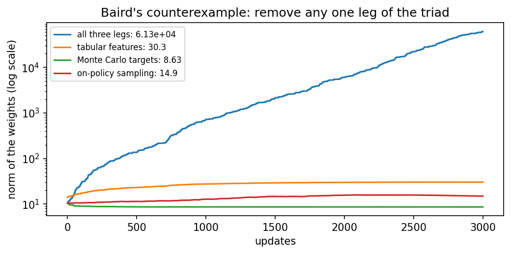
The vertical axis of the figure is logarithmic: Each labelled line stands for ten times the value of the line below, so a straight rising line means growth by a constant factor. With all three legs the norm climbs from 10.3 to \(6.13 \times 10^4\), which the legend writes as 6.13e+04. The estimated values of the seven states have then risen to between 70000 and 95000, although every true value is zero.
Each of the other runs removes one leg, and its curve stays flat. With tabular features every state has its own weight, \(\hat{V}_w(s) = w_s\), and nothing is shared. The norm rises from 14.1 to 30.3, because the six values of 3 move towards the value of the seventh state, and levels off. With Monte Carlo targets the bootstrapped target is replaced by the true return, zero. All values go to zero, and the norm ends at 8.63: Eight weights for seven states can give every state the value zero without being zero themselves. With on-policy sampling the agent follows the target policy itself, \(\rho = 1\), and the norm ends at 14.9.
Each leg is in use for a reason, so removing one has a price. Function approximation is needed when the states are too many for a table. Bootstrapping lets the agent learn before an episode ends and from less noisy targets. Off-policy learning lets it learn about the greedy policy while it explores, and from stored data, as experience replay does. A deep Q-network uses all three, and its two remedies make divergence less likely without ruling it out. Part A of the interactive lab runs Baird's counterexample in the browser, with a switch for each leg and a slider for the step size.
Python code in the Colab notebook, Section 7. Open Section 7 of the Colab notebook, which is optional, and run it. The function schedules trains Q-learning with one of the nine combinations, and the cell prints the table above. The function baird runs Baird's counterexample. Its options features="tabular", target="mc" and sampling="on-policy" each remove one leg of the triad, and the cell draws the figure shown here.
Python step 2: NumPy arrays and tables of values
Python code in the Colab notebook, right after Section 0 (setup). Open the notebook and run this step cell by cell: It consists of short pieces of Python code with their explanations, a quick check and three exercises. Topics: A table of values as an array · One temporal difference update · An environment as a function · Monte Carlo and temporal differences on the chain · The table, readable.
The notebook continues with the hands-on sections, and the interactive lab holds three practice parts and the self-assessment. The study path, the daily task and the research assignment are on the day overview.
Review cards
Select a card to turn it over.
References
[1] Sutton, R. S., & Barto, A. G. (2018). Reinforcement Learning: An Introduction (2nd ed.). MIT Press.
[2] Rummery, G. A., & Niranjan, M. (1994). On-line Q-learning using connectionist systems (Technical Report CUED/F-INFENG/TR 166). Cambridge University Engineering Department.
[3] Watkins, C. J. C. H., & Dayan, P. (1992). Q-learning. Machine Learning, 8(3-4), 279-292.
[4] Mnih, V., Kavukcuoglu, K., Silver, D., Rusu, A. A., Veness, J., Bellemare, M. G., Graves, A., Riedmiller, M., Fidjeland, A. K., Ostrovski, G., et al. (2015). Human-level control through deep reinforcement learning. Nature, 518(7540), 529-533. https://doi.org/10.1038/nature14236
[5] Lin, L.-J. (1992). Self-improving reactive agents based on reinforcement learning, planning and teaching. Machine Learning, 8(3-4), 293-321.
[6] Harris, C. R., Millman, K. J., van der Walt, S. J., Gommers, R., Virtanen, P., Cournapeau, D., Wieser, E., Taylor, J., Berg, S., Smith, N. J., et al. (2020). Array programming with NumPy. Nature, 585(7825), 357-362. https://doi.org/10.1038/s41586-020-2649-2
[7] McKinney, W. (2010). Data structures for statistical computing in Python. In Proceedings of the 9th Python in Science Conference (pp. 56-61). https://doi.org/10.25080/Majora-92bf1922-00a
[8] Bellman, R. (1957). A Markovian decision process. Journal of Mathematics and Mechanics, 6(5), 679-684.
[9] van Hasselt, H., Guez, A., & Silver, D. (2016). Deep reinforcement learning with double Q-learning. In Proceedings of the AAAI Conference on Artificial Intelligence, 30(1), 2094-2100.